Documentation
Arnodiqa is a desktop application for Windows. This documentation explains, task by task, how to work in the app, with the steps, screenshots and a short recording. For test benches without a screen and for pipelines there is the command line, described under Automation and CI.
Creating a project, starting a measurement, the Trace with a filter, a frame with signals and a signal in Graphics.
The main window
| Toolbar | Project menu, Start and Stop (F9, Esc), state and measurement time, the working mode (simulated bus, real bus or offline), the command search (Ctrl+K), bus load per channel, Help and theme. |
|---|---|
| Desktops | Analysis (Trace and Write), Messages, Signals (Graphics, Data, Statistics), Stimulation (Interactive Generator) and Project (project explorer and simulation setup). |
| Windows | Window adds windows. Windows can be dragged and docked; Layout saves the arrangement. |
| Write window | Messages from the system, from scripts (Program tab) and from tests (Test tab). |
| Status bar | State, connection to the engine, number of events, events per second, buffer and logging. |
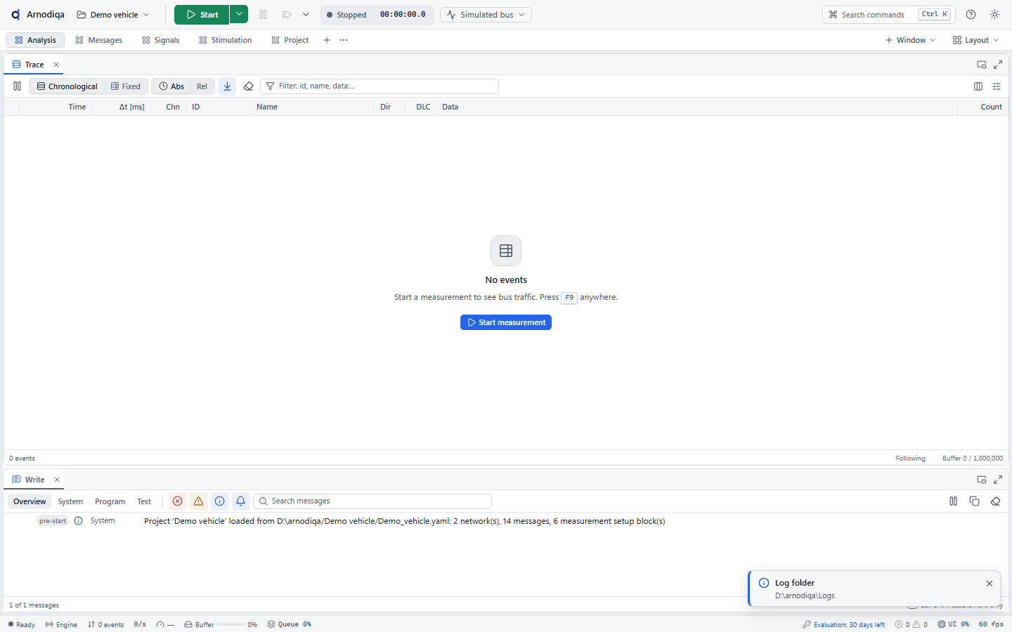
Screenshots and recordings follow the theme of this site. Click an image to enlarge it.
Open a project, create a new one and add a database
A project bundles the networks, databases, measurement setup, panels and simulation nodes in one YAML file.
Without a loaded project, Arnodiqa opens the start page (Start). New project lists the templates, Examples the examples and Recent projects the projects used last.
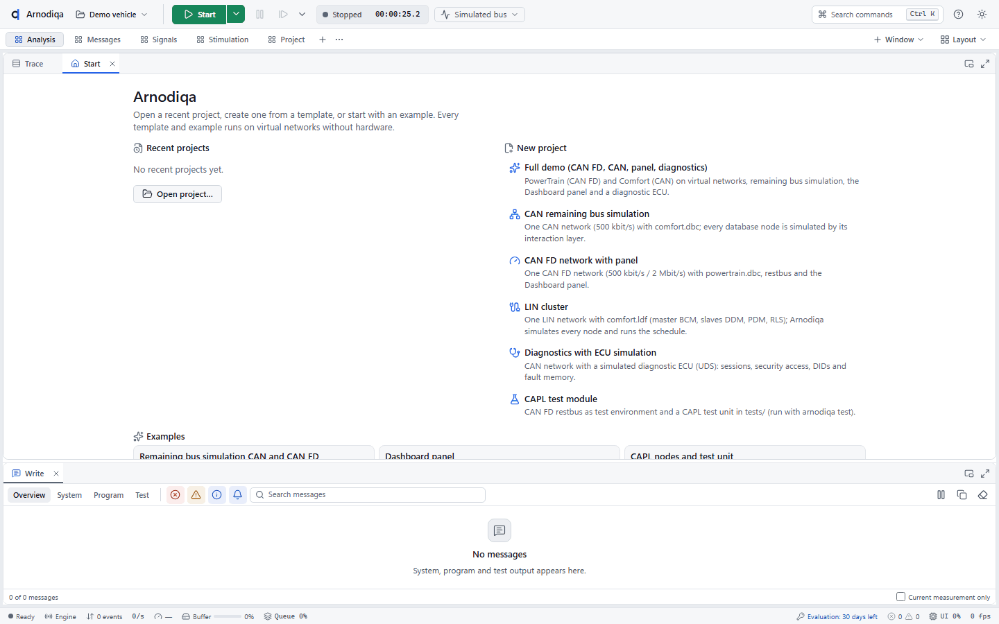
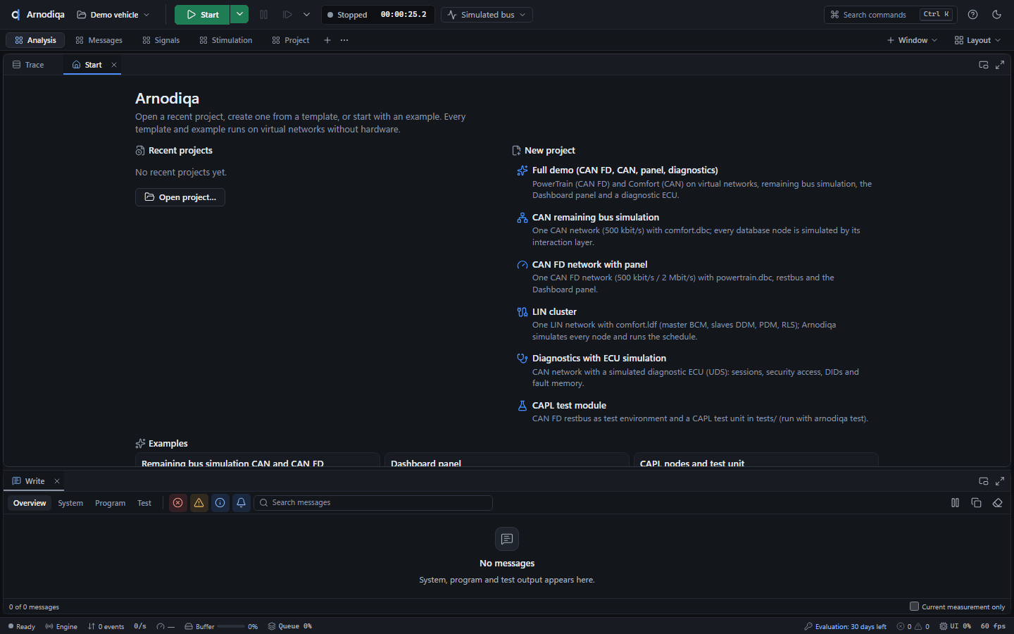
Click the project menu at the top left (the button with the project name; without a project it reads No project). Choose New project… for a new project or Open project… (Ctrl+O) to open an existing project file (.yaml).
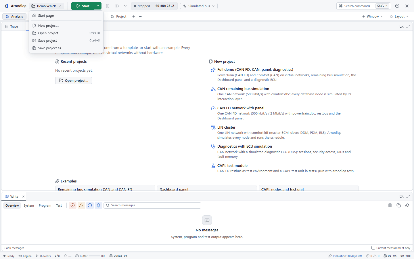
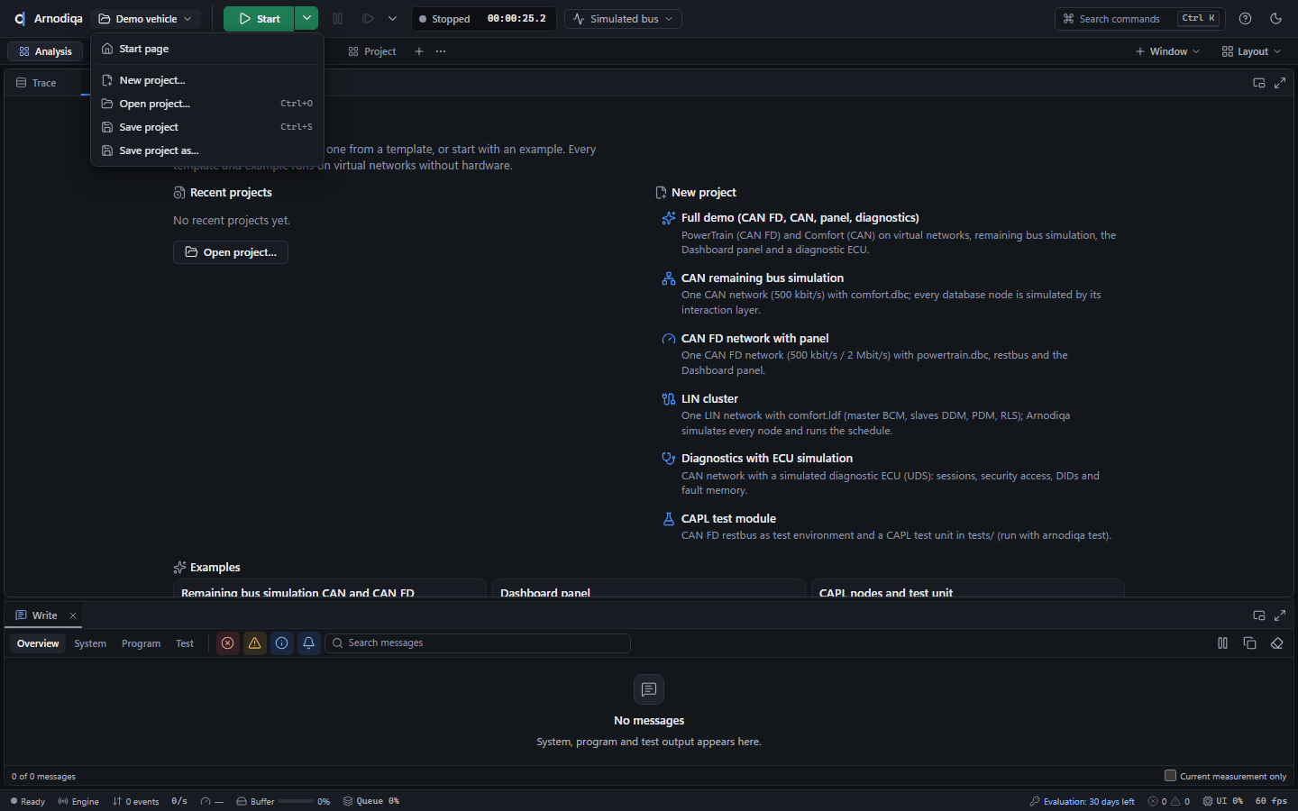
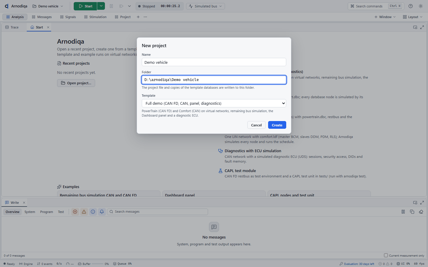
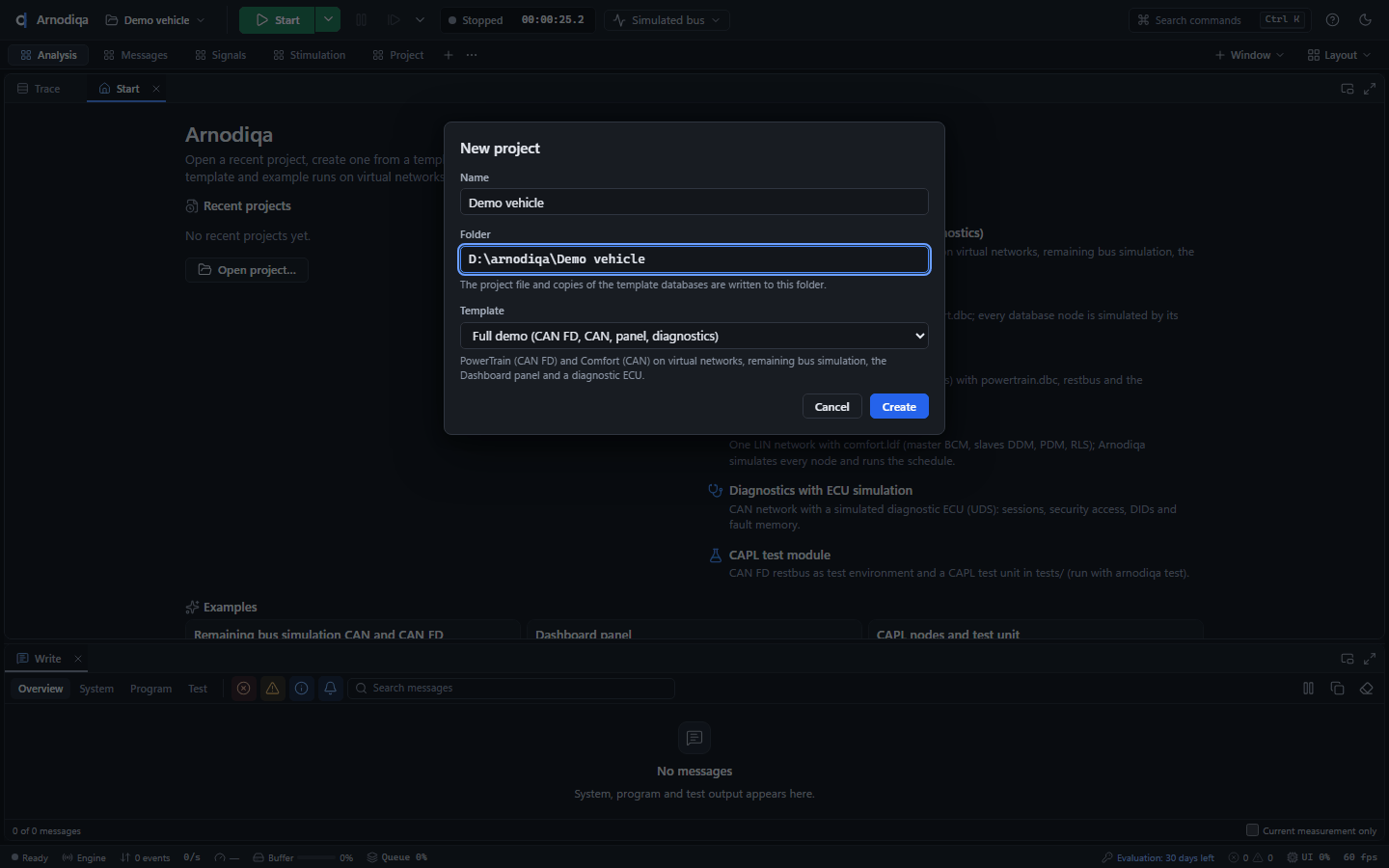
In the New project dialog, enter the project name under Name, choose the project folder under Folder (with Browse…) and a template under Template, for example Full demo (CAN FD, CAN, panel, diagnostics). Click Create.
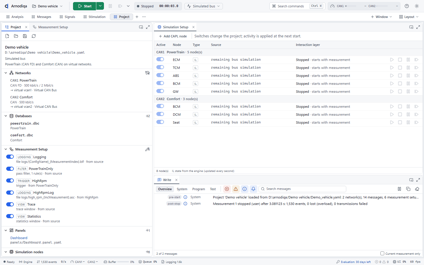
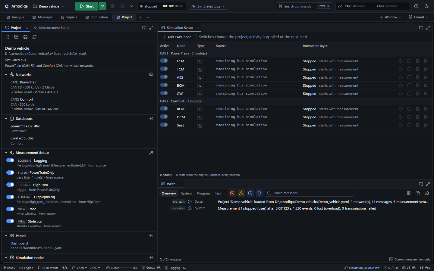
The project is loaded and its name appears in the toolbar. On the Project desktop, the project explorer shows the networks, databases, measurement setup, panels and simulation nodes; the simulation setup is on the right.
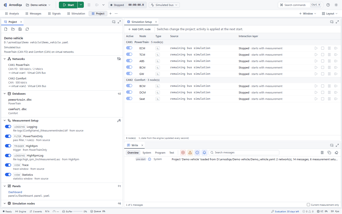
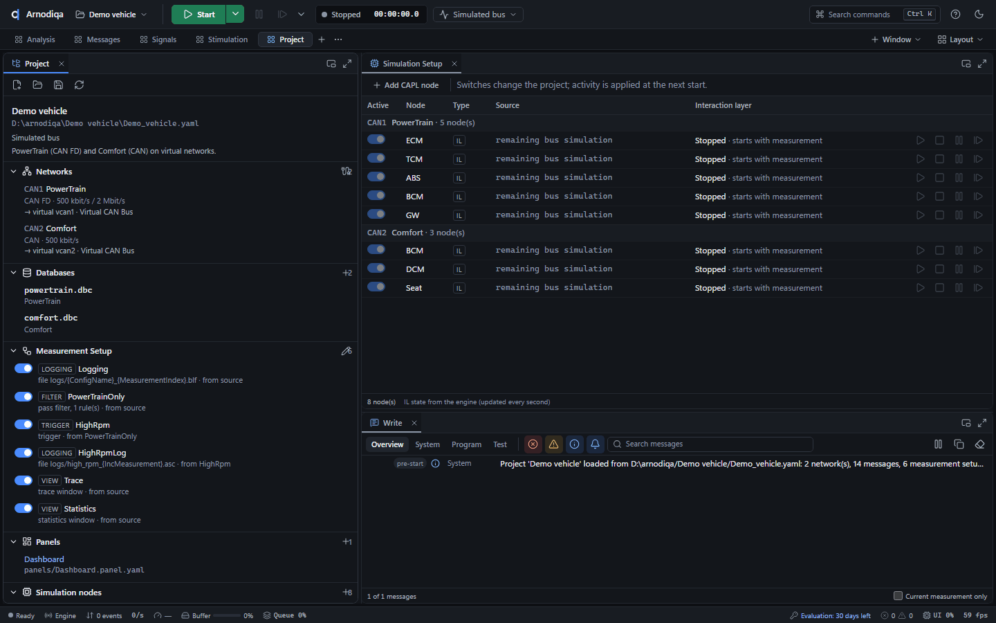
The project's databases are listed under Databases, here powertrain.dbc for PowerTrain and comfort.dbc for Comfort. The pencil next to a DBC or LDF file opens the Database Editor; the bin removes the database from the project, the file itself remains.
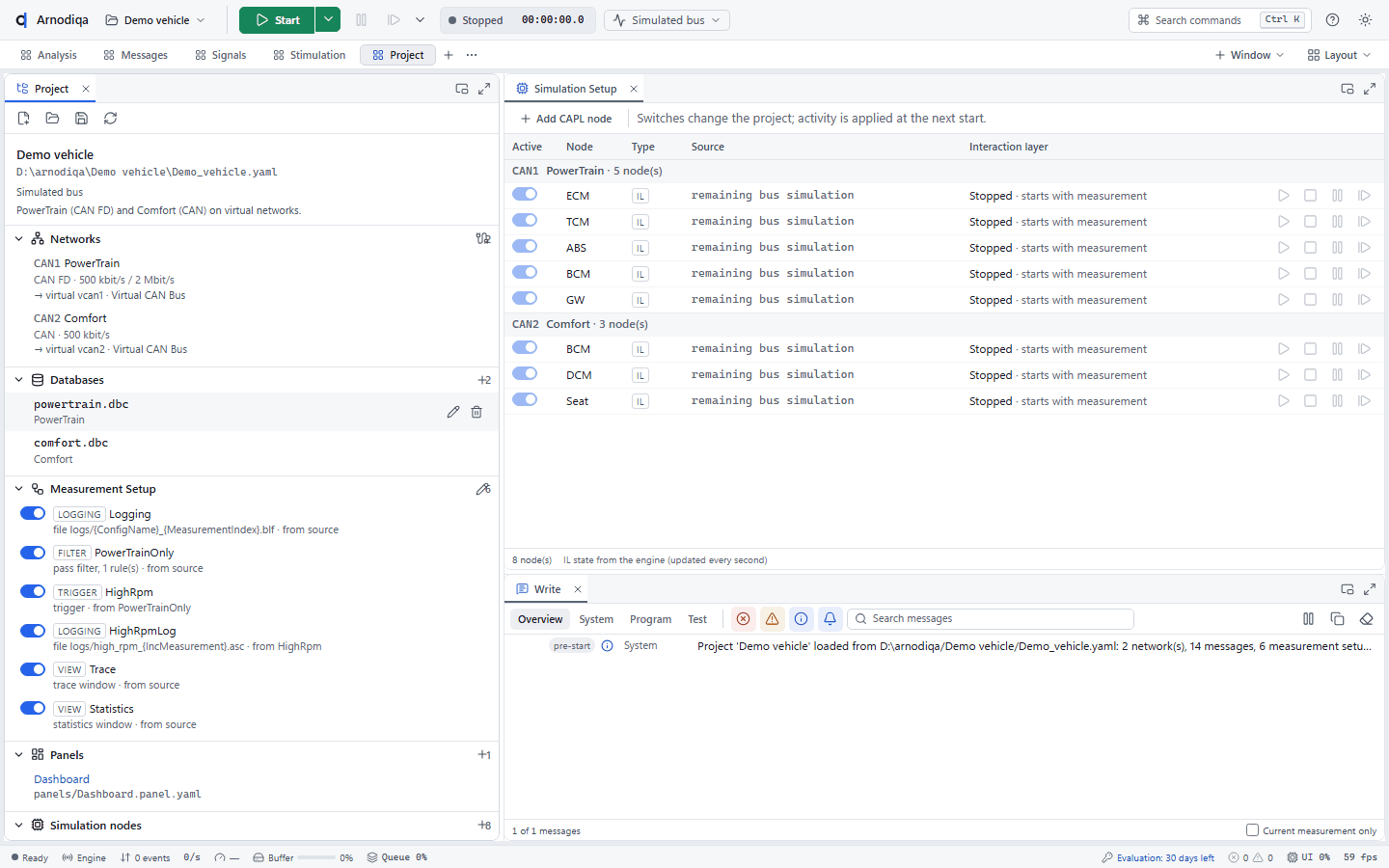
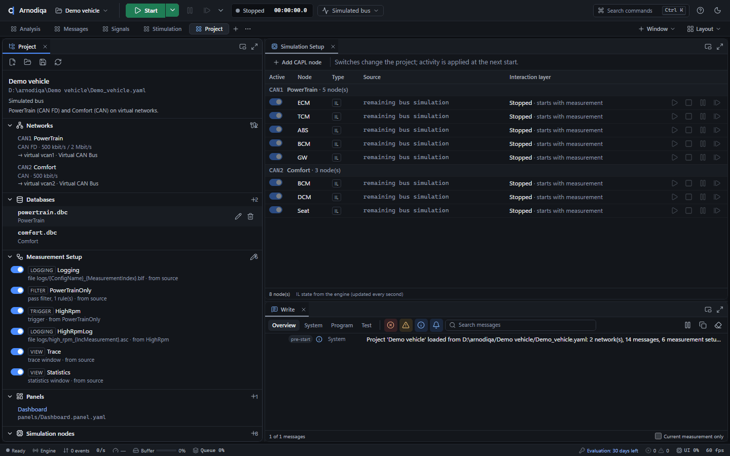
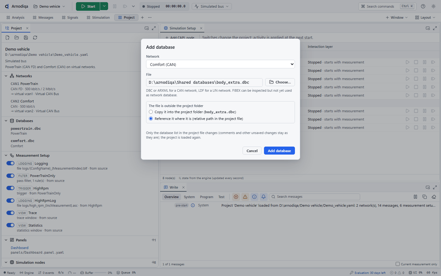
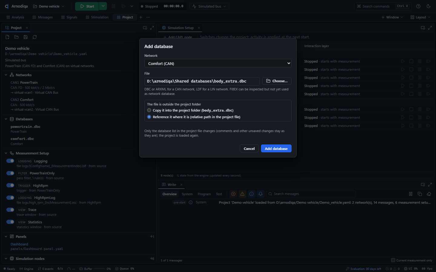
To add a database, click the + to the right of Databases or the + next to a network. In Add database, choose the network (here Comfort), click Choose… and select a DBC, LDF (for a LIN network), ARXML or FIBEX file.
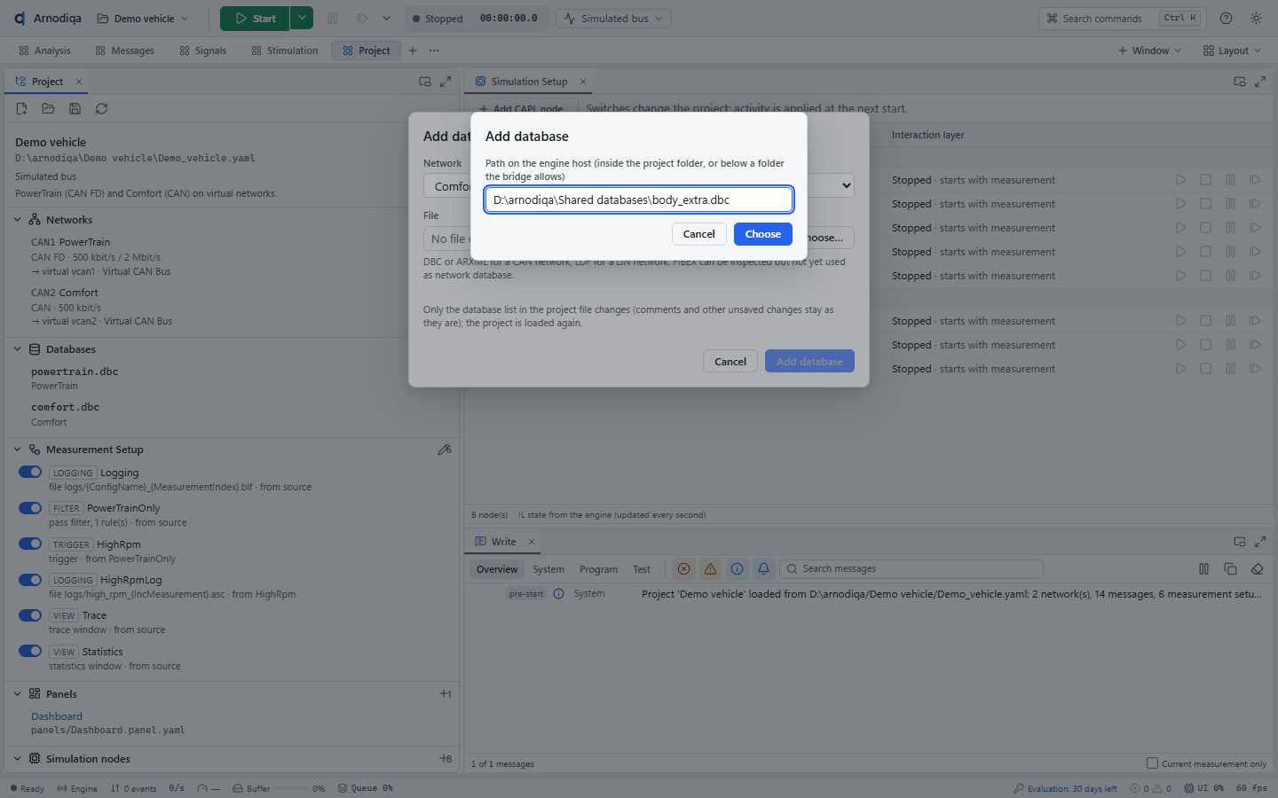
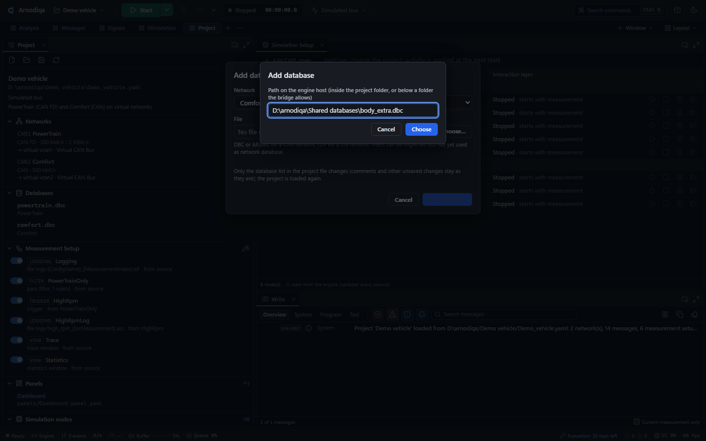
If the file is outside the project folder, choose Copy it into the project folder (a copy next to the project file) or Reference it where it is (the project refers to the file with a relative path, for example ../Shared databases/body_extra.dbc). Click Add database.
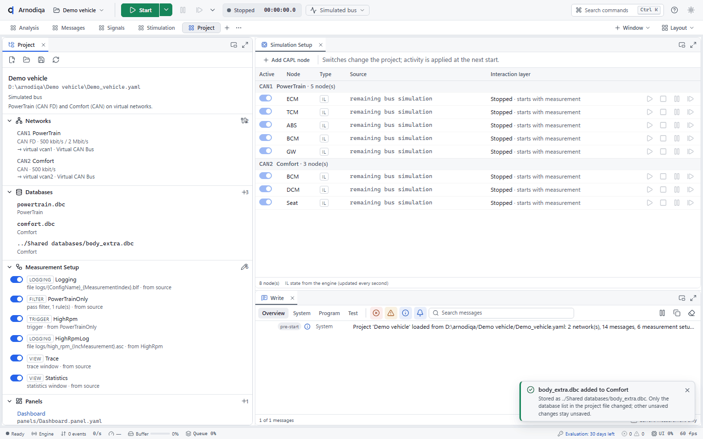
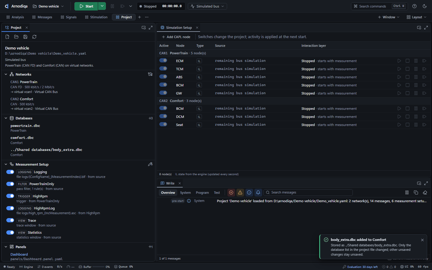
Arnodiqa saves and reloads the project: the database appears under Databases for Comfort, and Trace, Data and Graphics know its messages immediately.
Select hardware or use the virtual bus
Each network of the project is assigned to a channel: a channel of an interface or of the virtual bus.
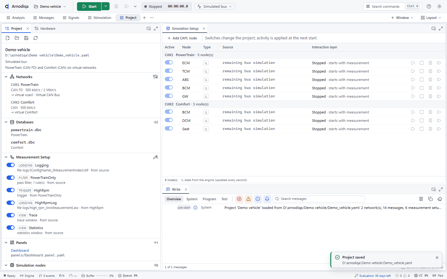
On the Project desktop, the project explorer shows the assignment of each network under Networks, for example → virtual vcan1 · Virtual CAN Bus. Click the Hardware configuration icon to the right of Networks.
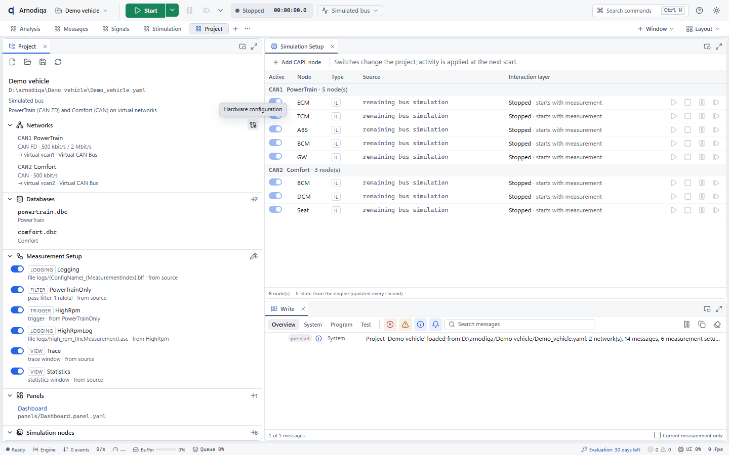
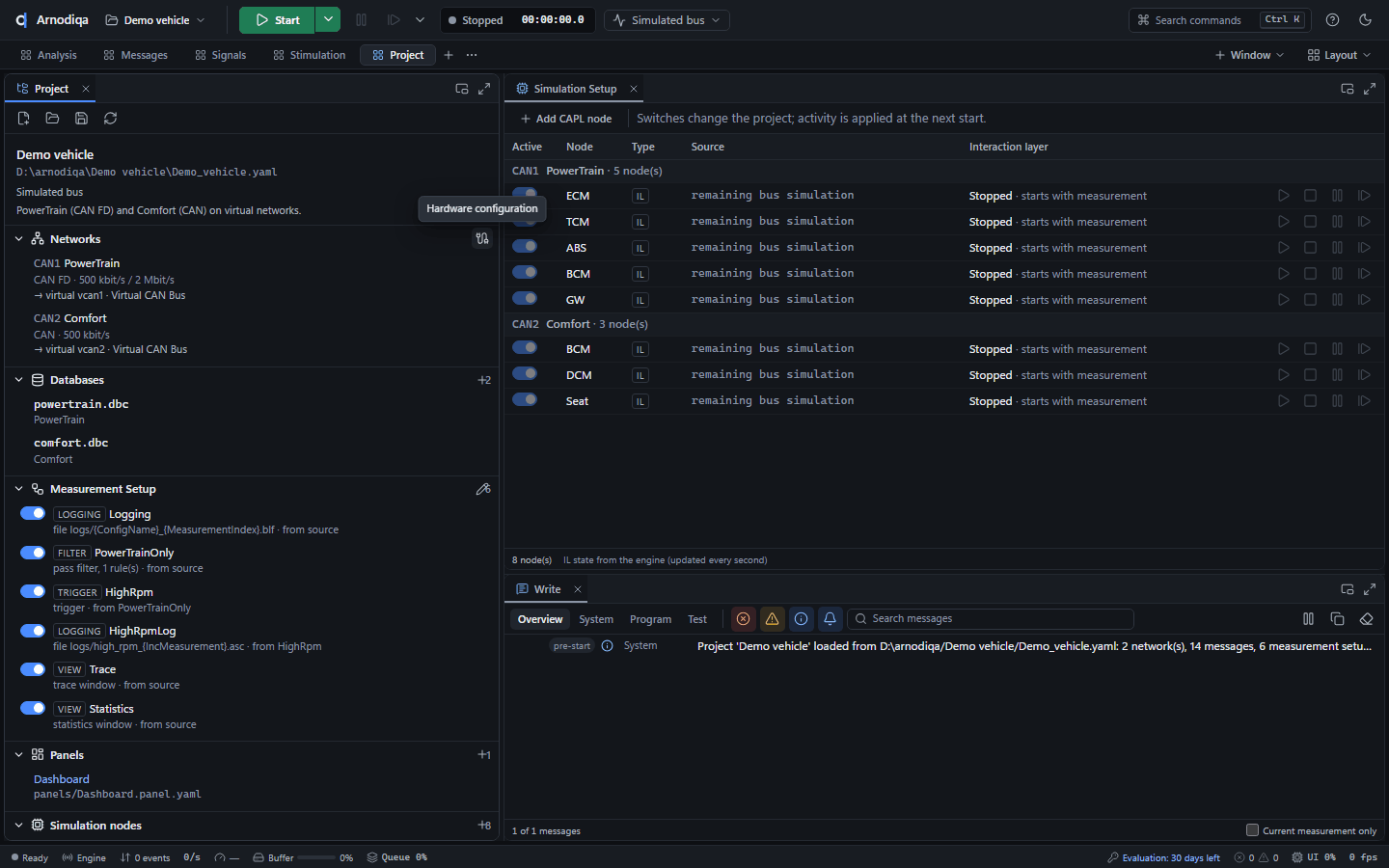
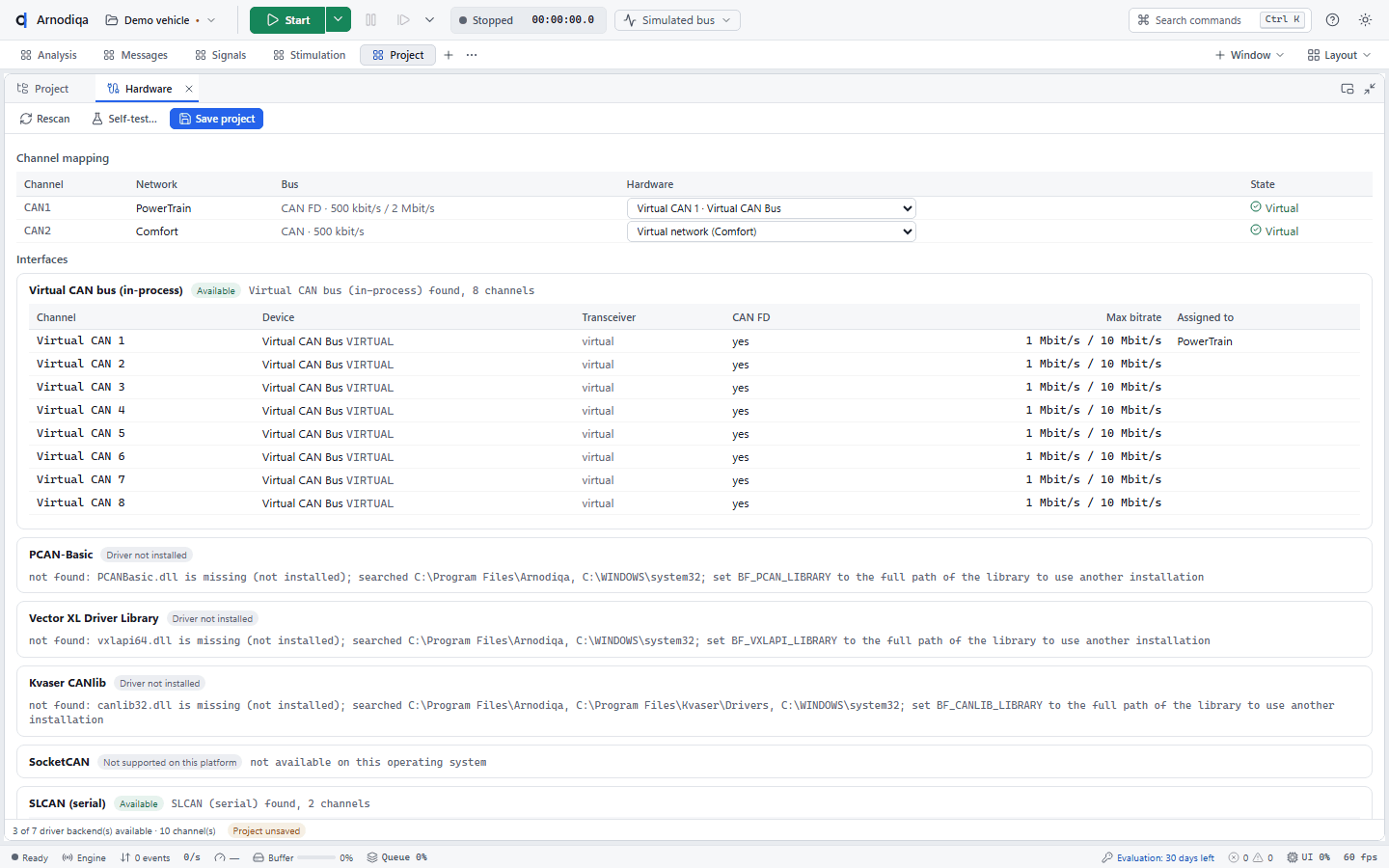
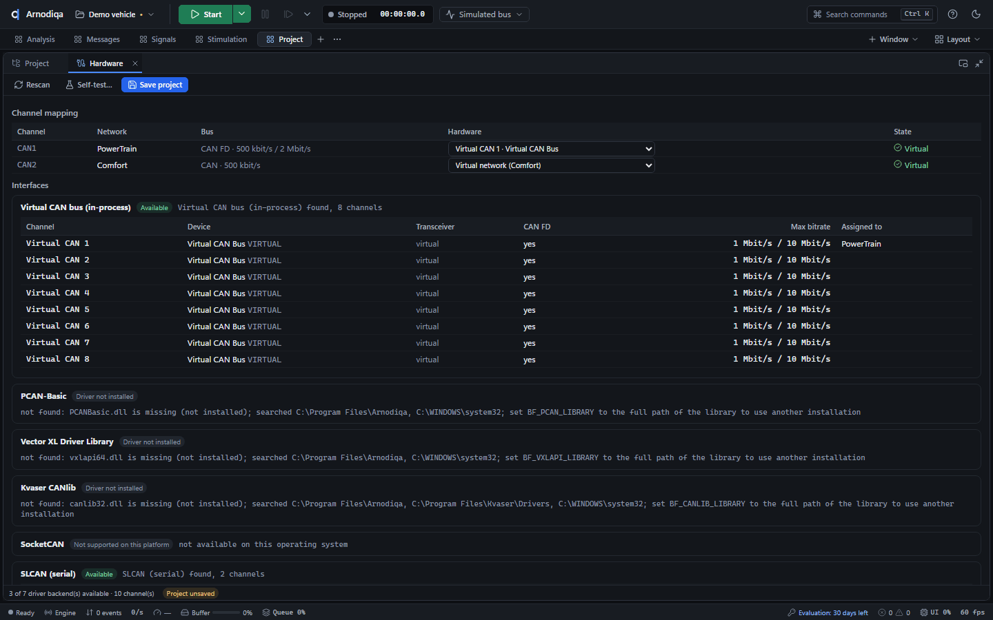
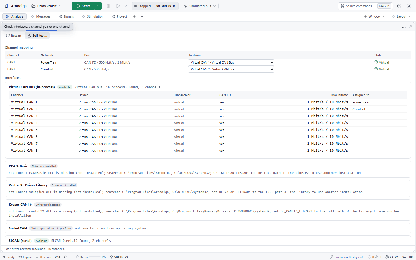
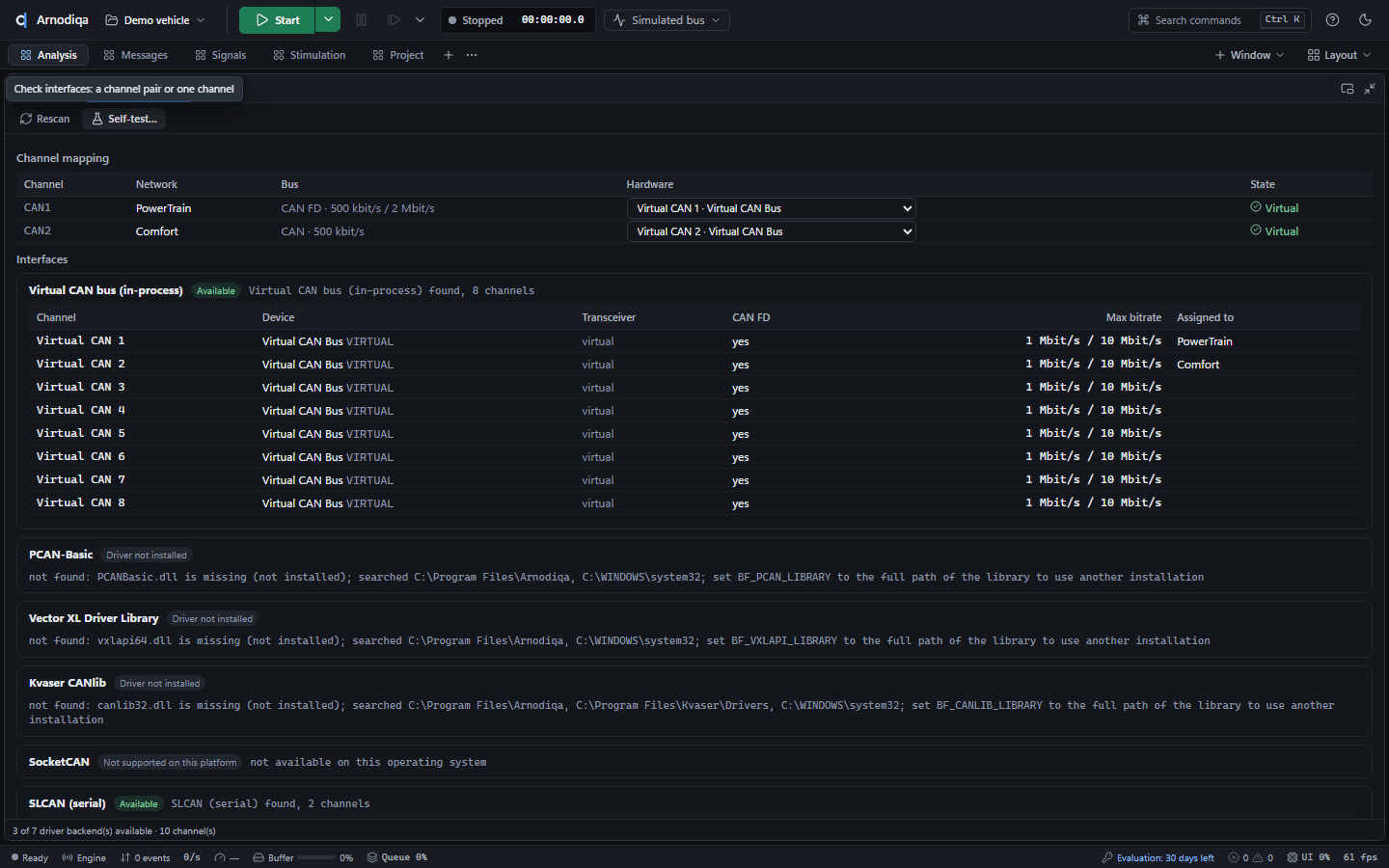
The Hardware window shows, under Channel mapping, the channel (column Hardware) and status of each network, and under Interfaces, for each driver whether it is available and which channels it found. Click Rescan after connecting an interface.
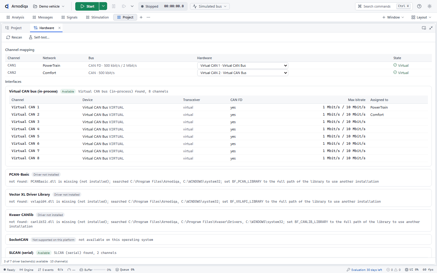
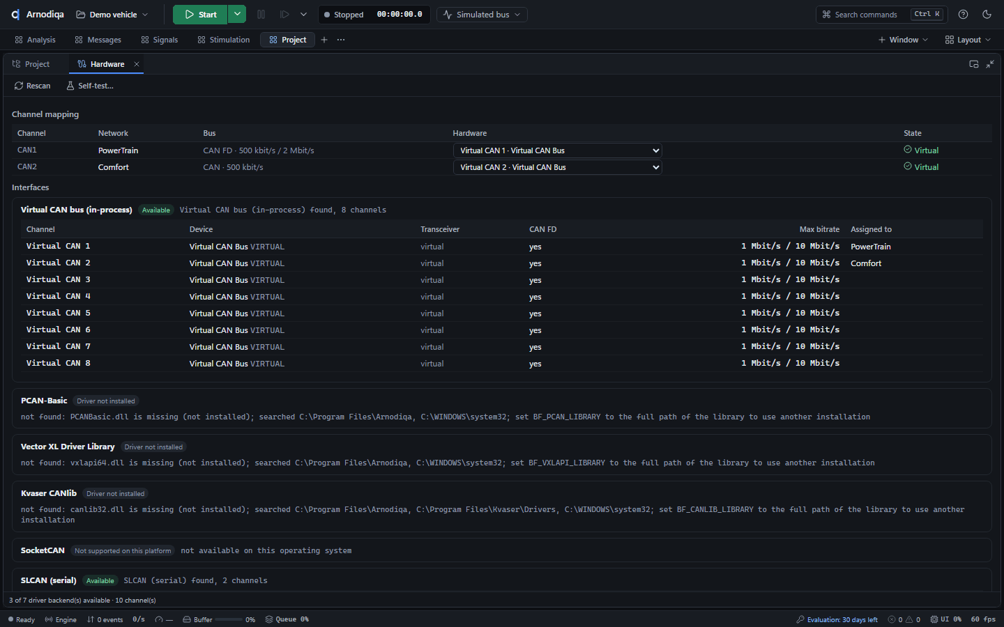
For each network, choose in the list under Hardware a channel of a connected interface, a channel of the virtual bus (Virtual CAN 1 …) or Virtual network (Comfort). The assignment applies immediately; click Save project to update the project file.
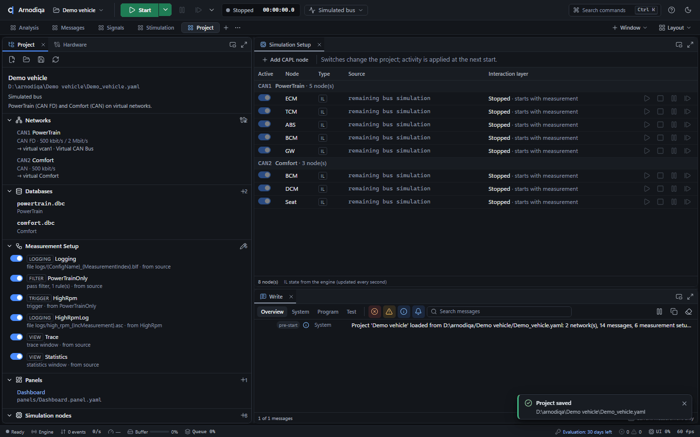
The project explorer shows the new assignment next to the network (→ virtual Comfort). A channel that is not found at start is shown there as not connected.
Start and stop a measurement
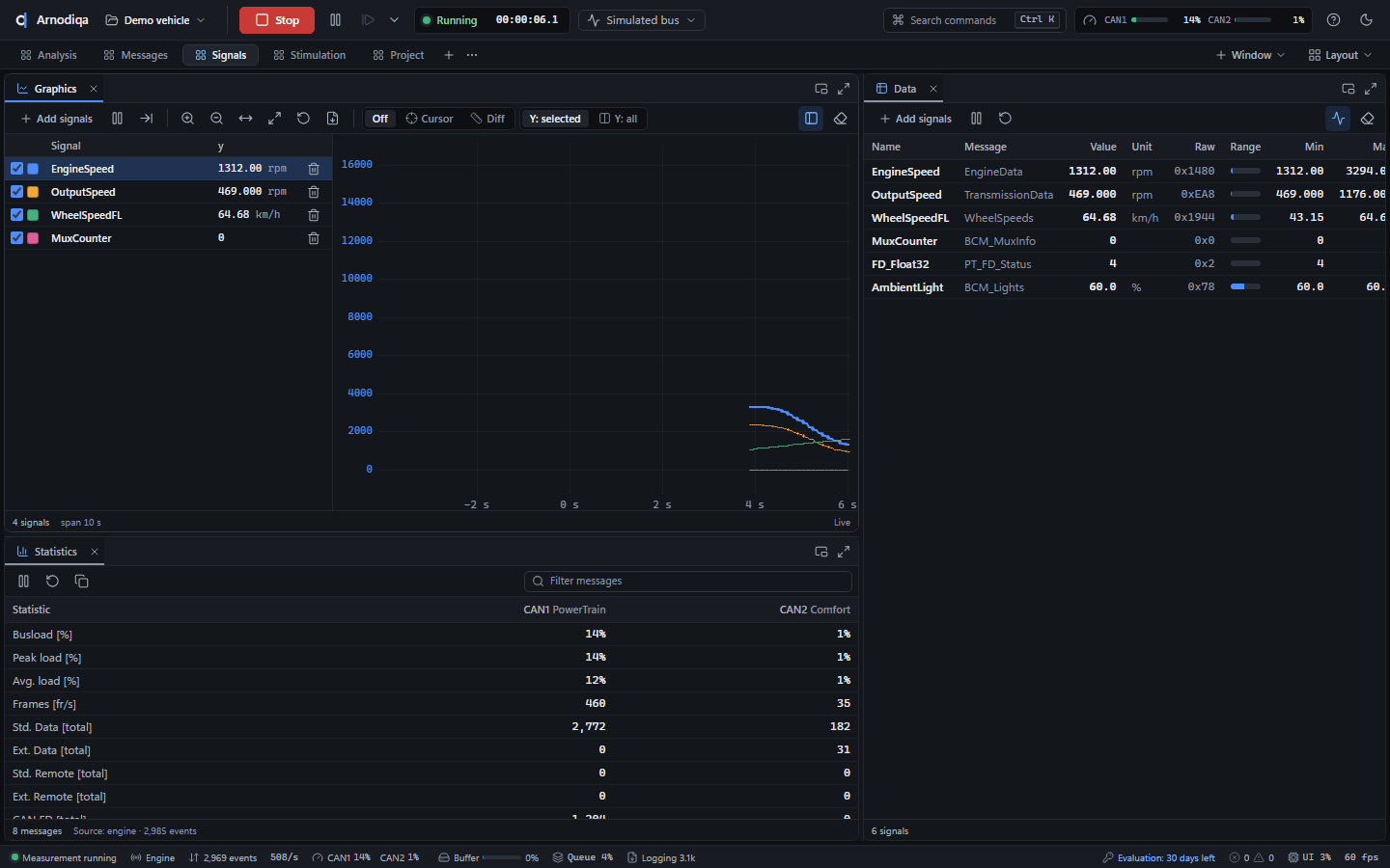
The toolbar, status bar and the Statistics window show the state of the measurement and the bus load.
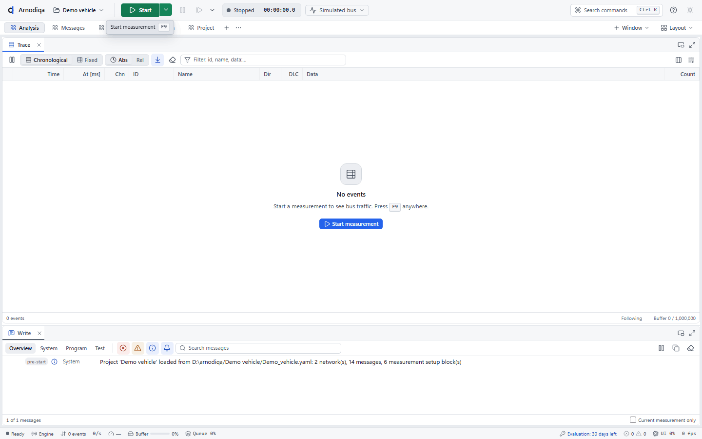
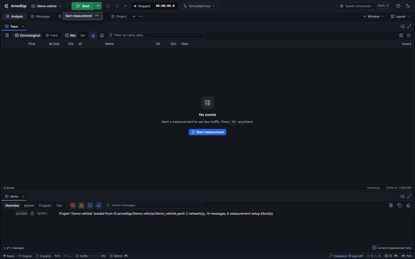
Click Start in the toolbar or press F9. The arrow next to Start offers Start measurement without logging.
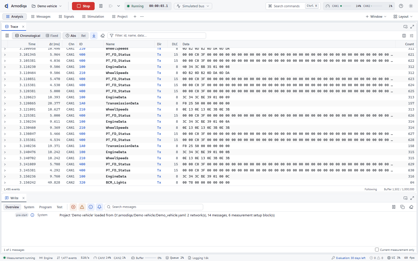
During the measurement the state shows Running with the measurement time, followed by the bus load per channel. The Trace fills up. The status bar at the bottom shows the number of events, events per second and the buffer level.
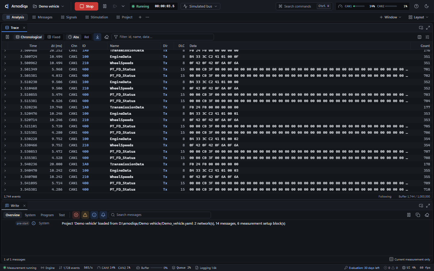
The bus load appears in the toolbar and in the status bar. The Statistics window on the Signals desktop gives more detail: per channel Busload [%], Peak load [%], frames per second and the frame counters. All three use the same calculation over a one-second window.
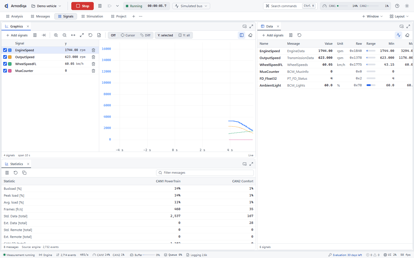
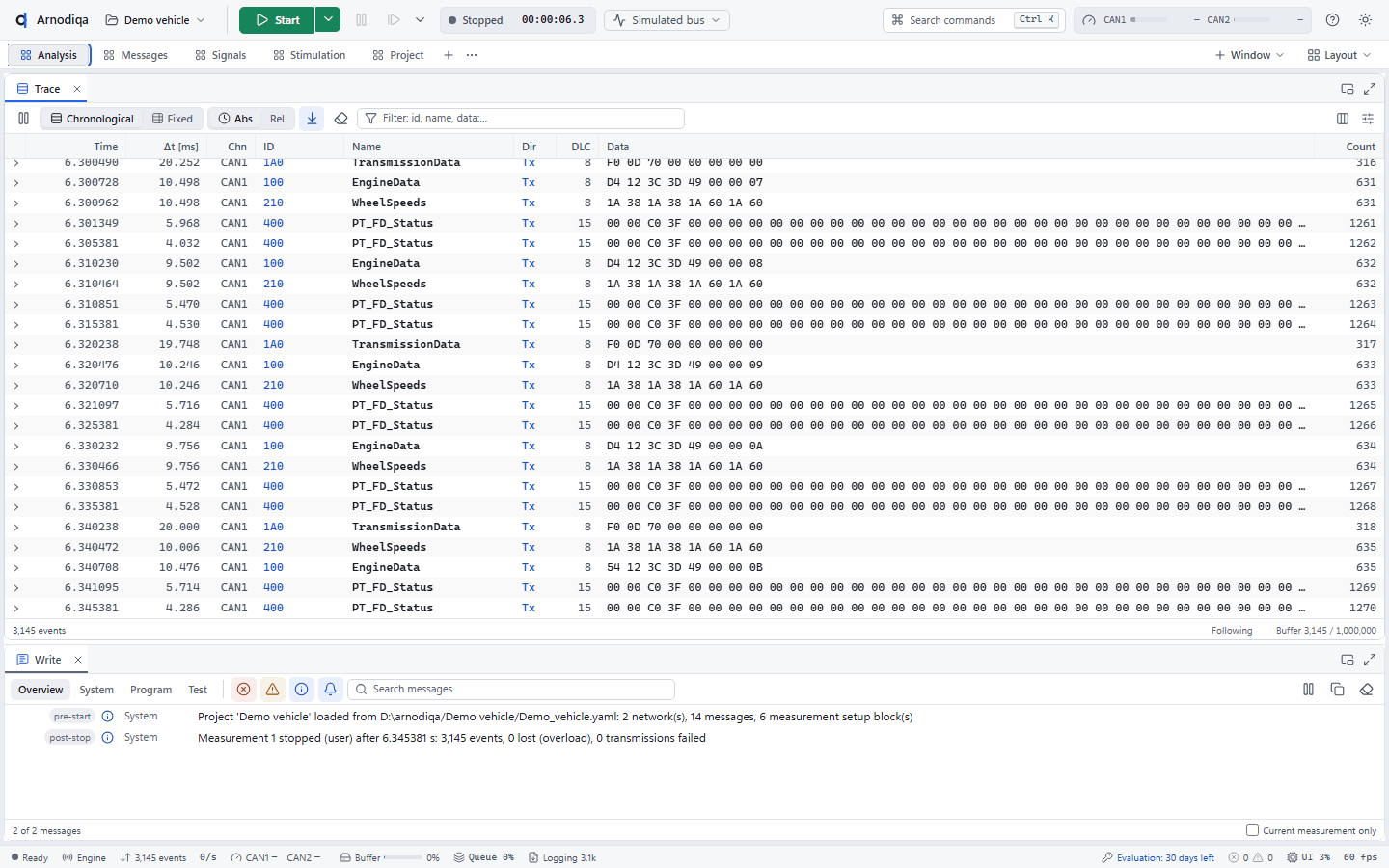
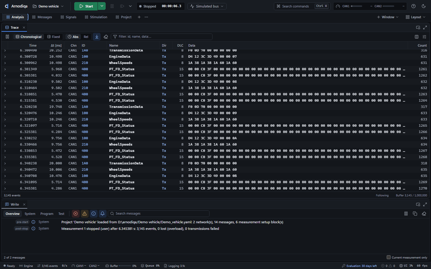
Stop the measurement with Stop or Esc. The Write window reports Measurement 1 stopped (user) after … s.
The Trace: modes, filtering, signals and export
The Trace shows every frame and bus event, decoded with the project's databases.
The Trace is on the Analysis desktop. In Chronological mode each event has its own row, newest at the bottom. Maximize at the top right makes the window fill the desktop.
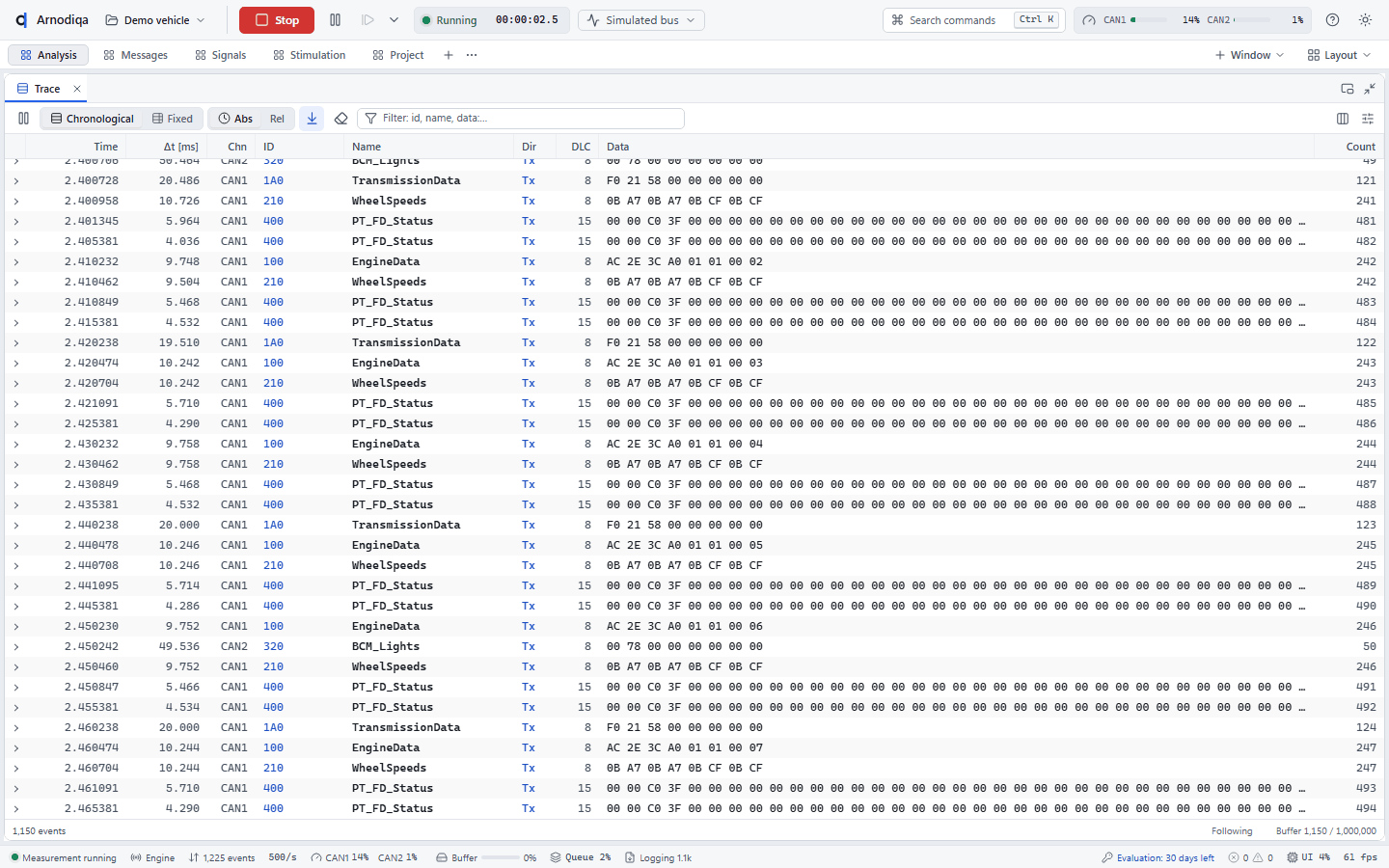
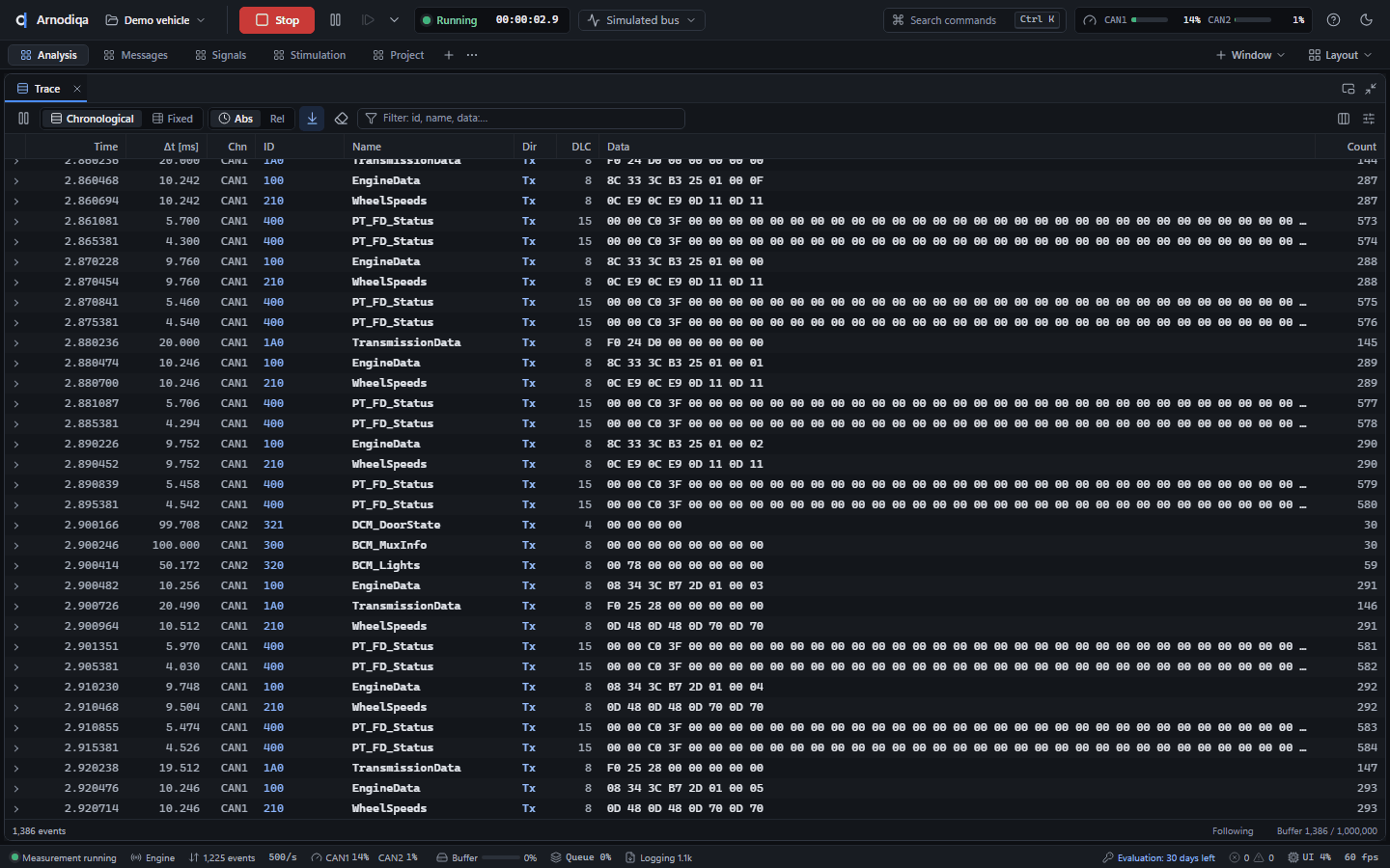
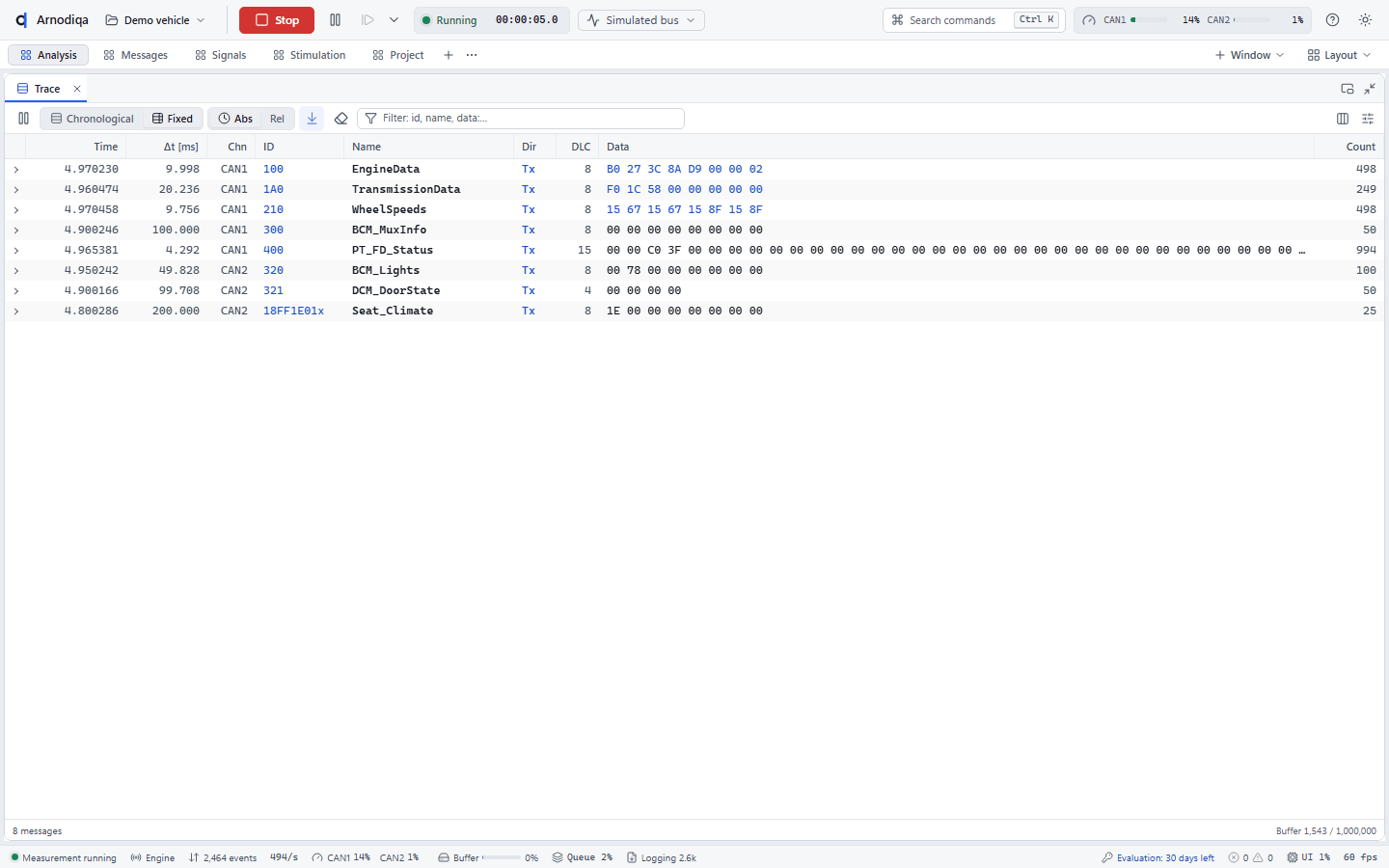
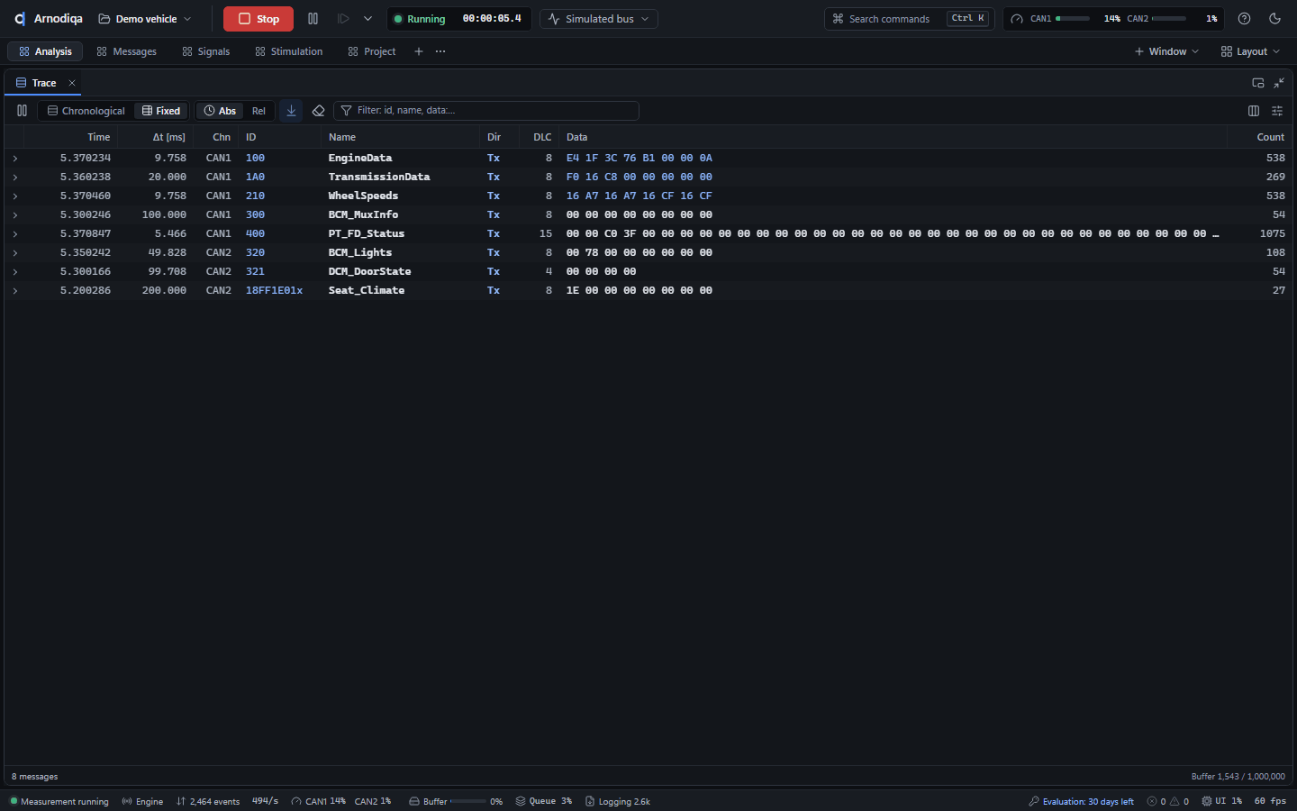
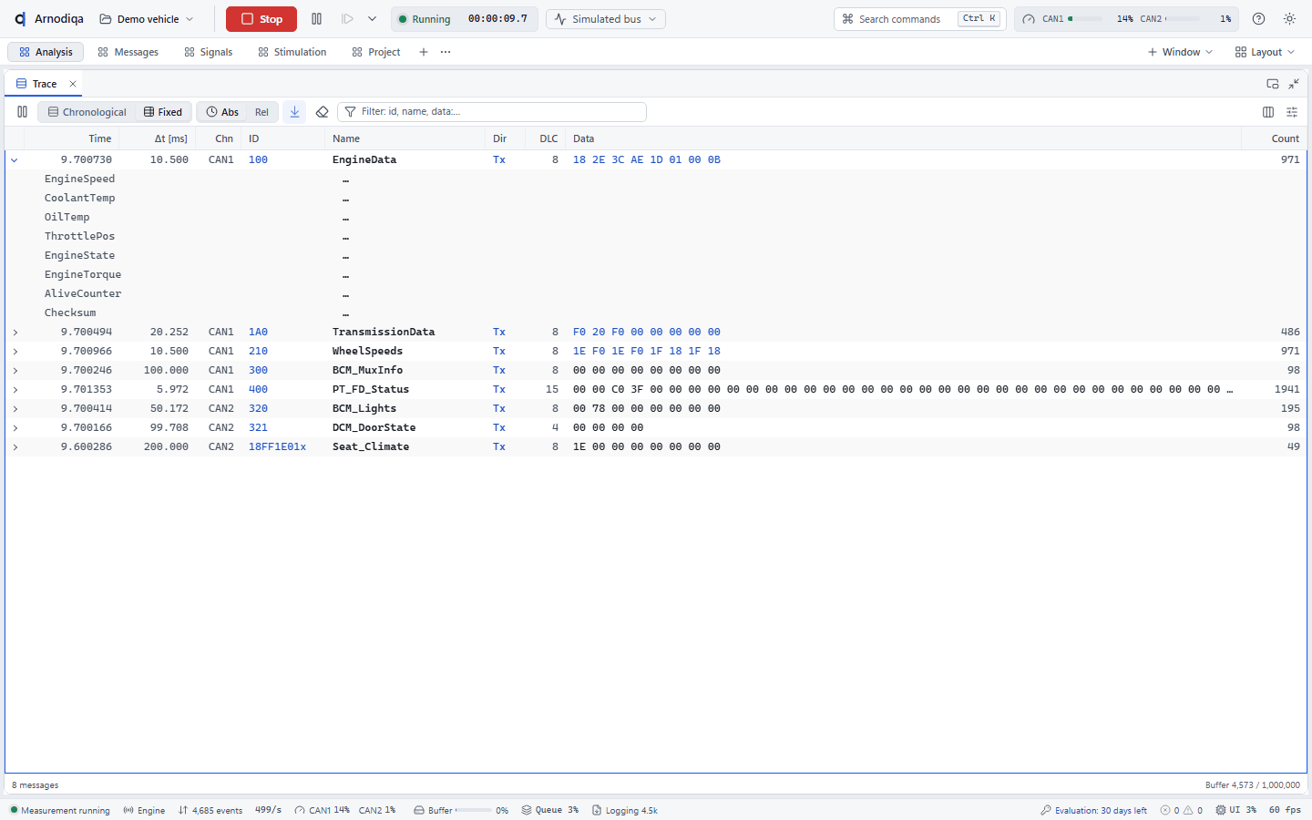
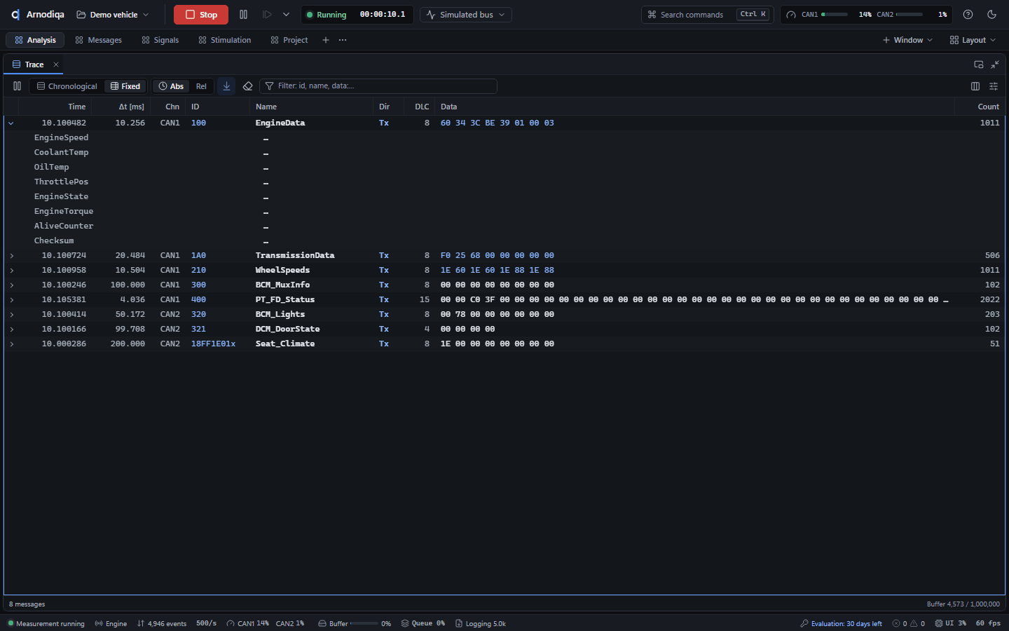
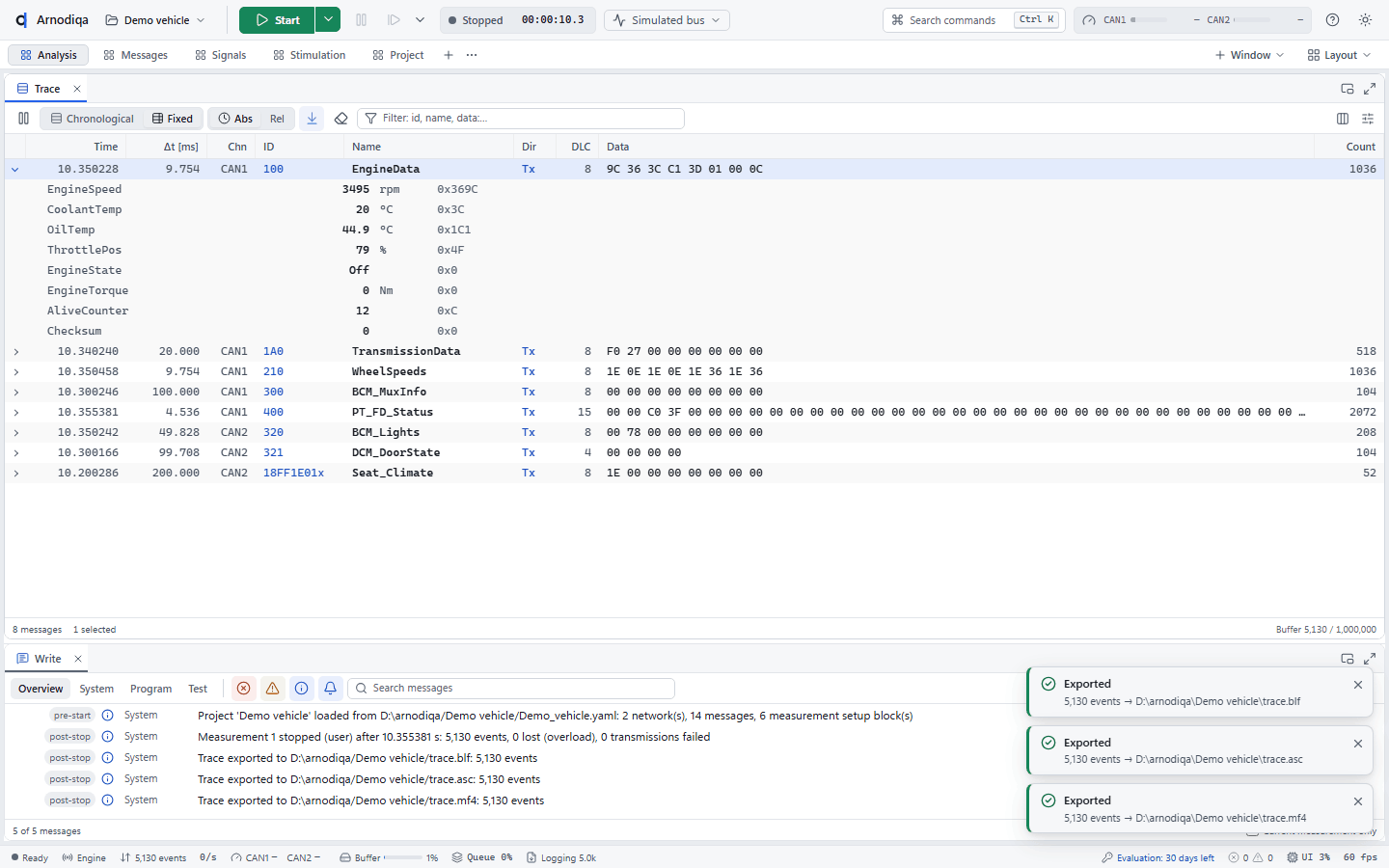
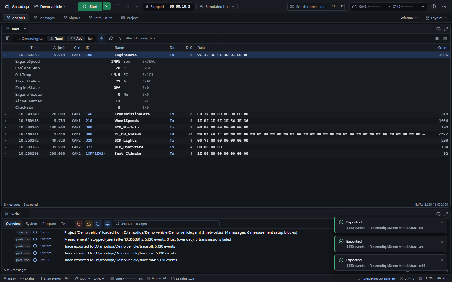
Click Fixed for one row per message, updated in place. Abs and Rel select absolute or relative time; Space pauses the display.
Type a filter in the filter field (Ctrl+F), here
name:Engine. Examples:1A0orid:100-1FF(ID or range),ch:CAN2orch:Comfort(channel or network),dir:tx,type:fd,!name:Door(not). Terms are combined; the field's tooltip shows the full syntax.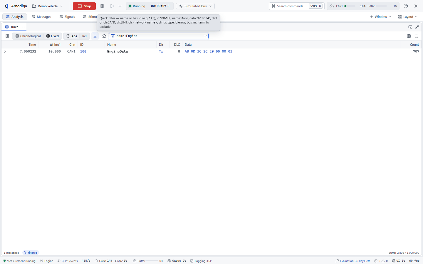
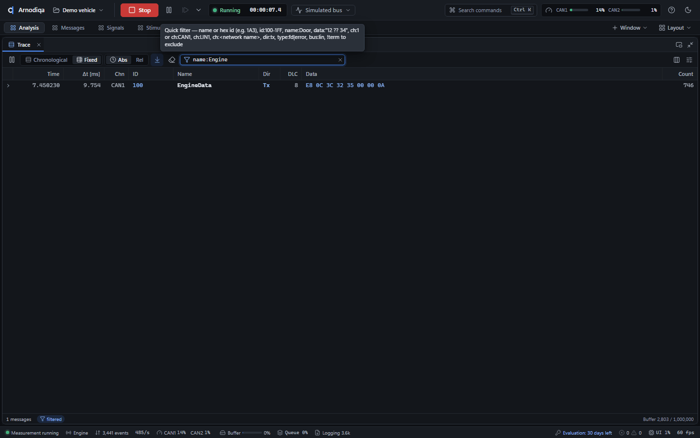
A second example:
ch:Comfort !name:Doorshows all messages on the Comfort network except those with Door in the name. The bottom bar shows filtered; Esc in the field clears the filter.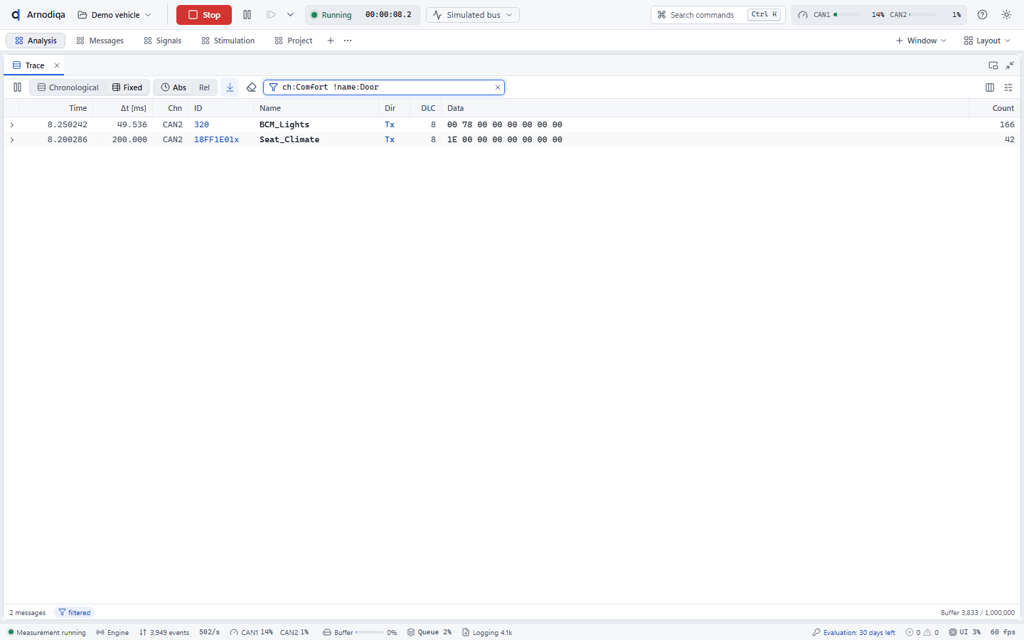
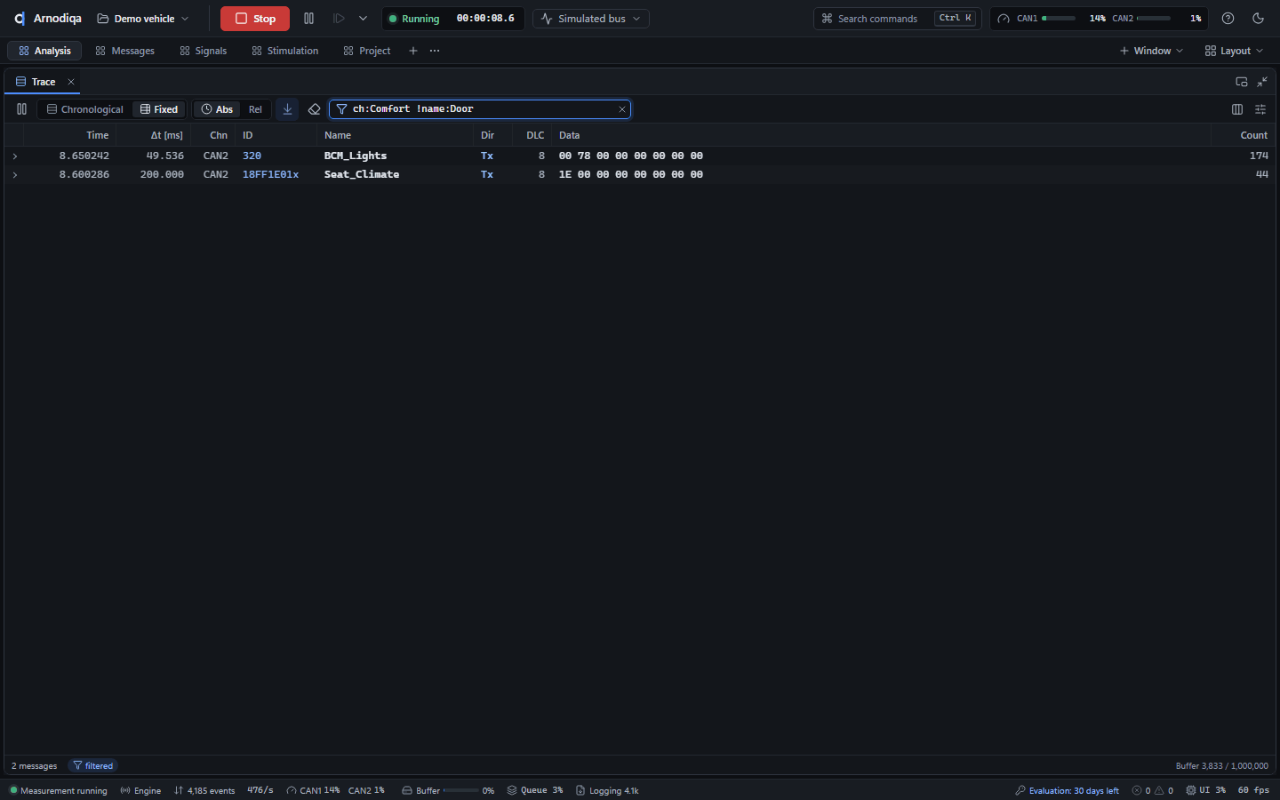
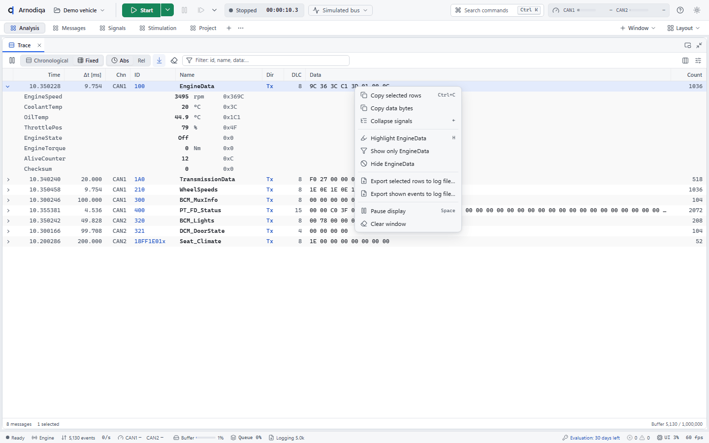
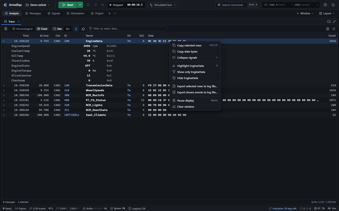
Click the arrow at the start of a row to expand the frame: each signal is listed below it with physical value, unit and raw value.
The context menu (right-click) contains Export selected rows to log file… and Export shown events to log file… (everything the window shows with the current filter). In the save dialog, choose the name and type: BLF, ASC, MF4 or PCAPNG.
After exporting, Arnodiqa reports the number of events written; the Write window lists each file, here trace.blf, trace.asc and trace.mf4.
Follow signals in Data and Graphics
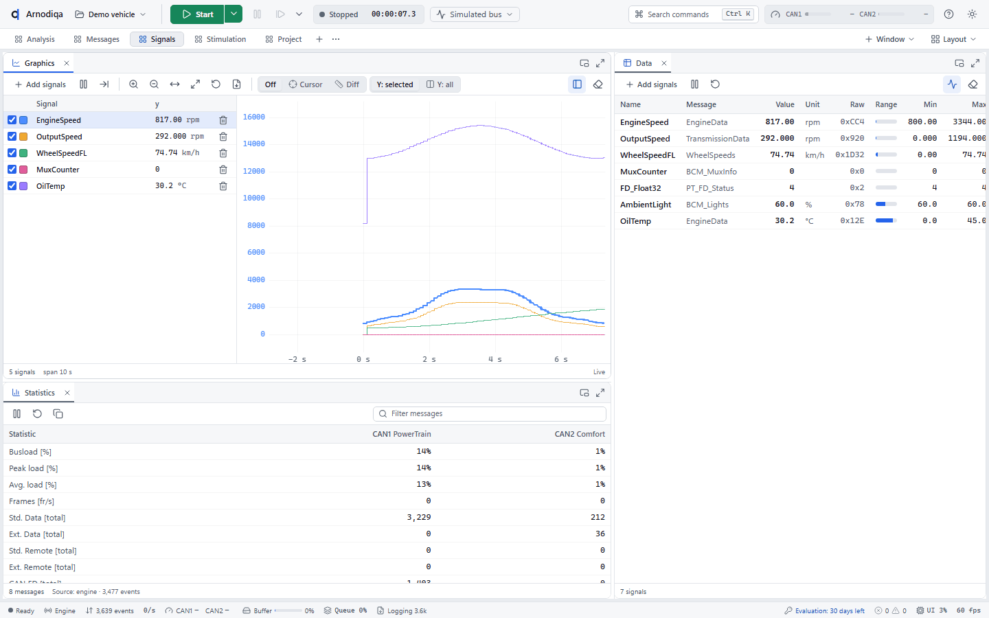
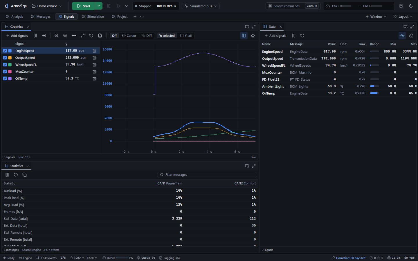
Data shows current signal values, Graphics their course over time.
Open the Signals desktop. Graphics and Data already contain signals from the project's databases.
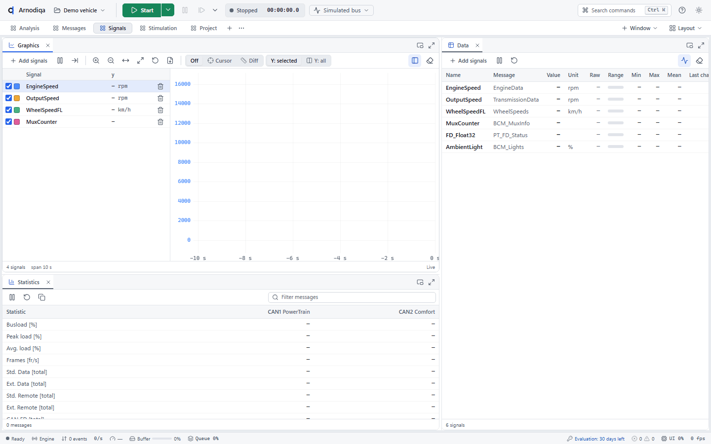
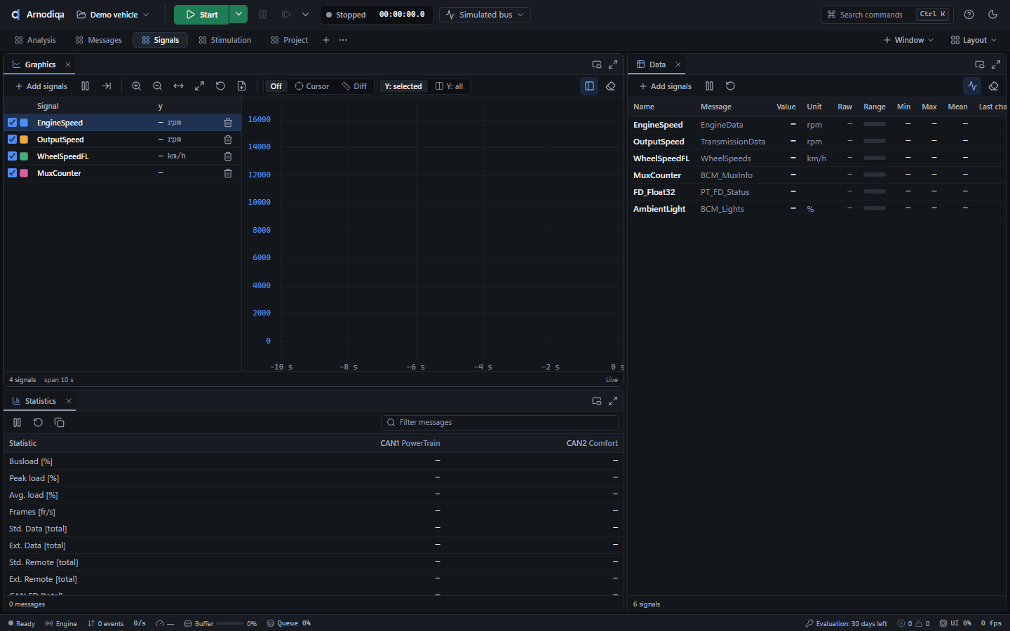
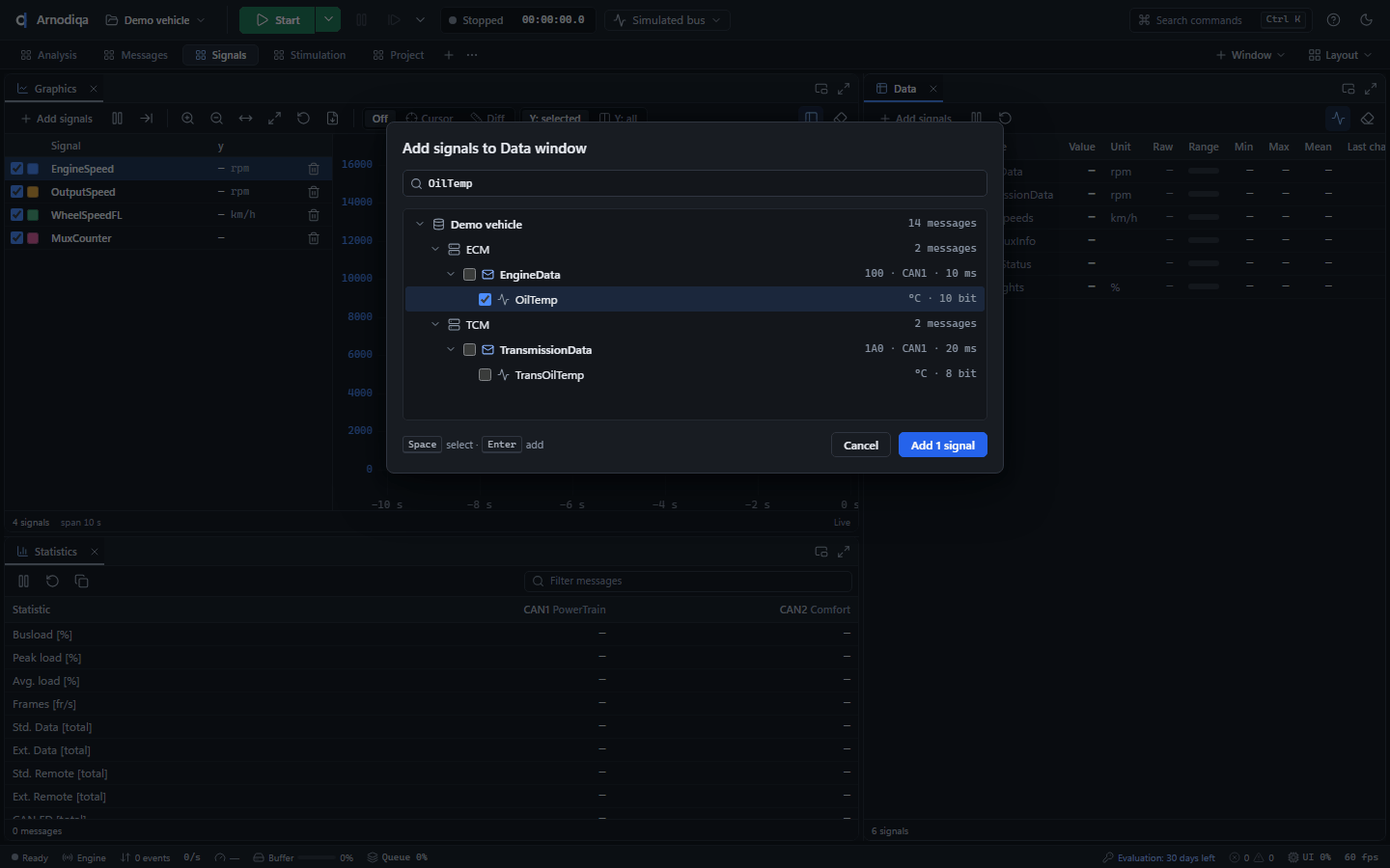
In the Data window, click Add signals. In Add signals to Data window, search by name (here OilTemp), tick the signal (Space) and click Add 1 signal (Enter). You can also drag a signal from the Trace into the window.
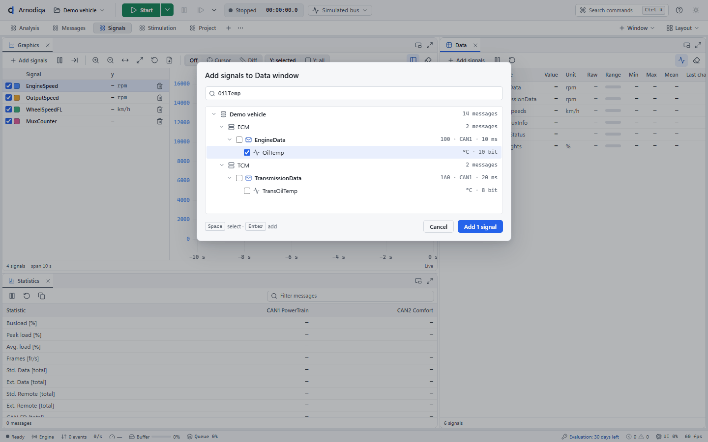
Do the same in Graphics with Add signals and start the measurement (F9). Data shows the current value, unit, raw value and min/max of each signal; Graphics shows the course over time with the latest value in the signal list.
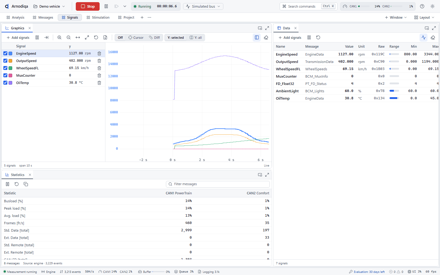
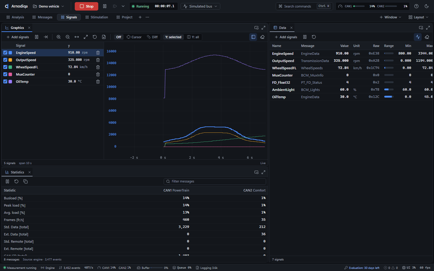
After stopping, the plot remains. Scroll in Graphics to zoom and drag to pan; the context menu exports the frames to a log file or the signals as CSV.
Send messages with the Interactive Generator
The Interactive Generator sends frames once, periodically or on a key.
The Stimulation desktop contains the Interactive Generator with messages from the project's database.
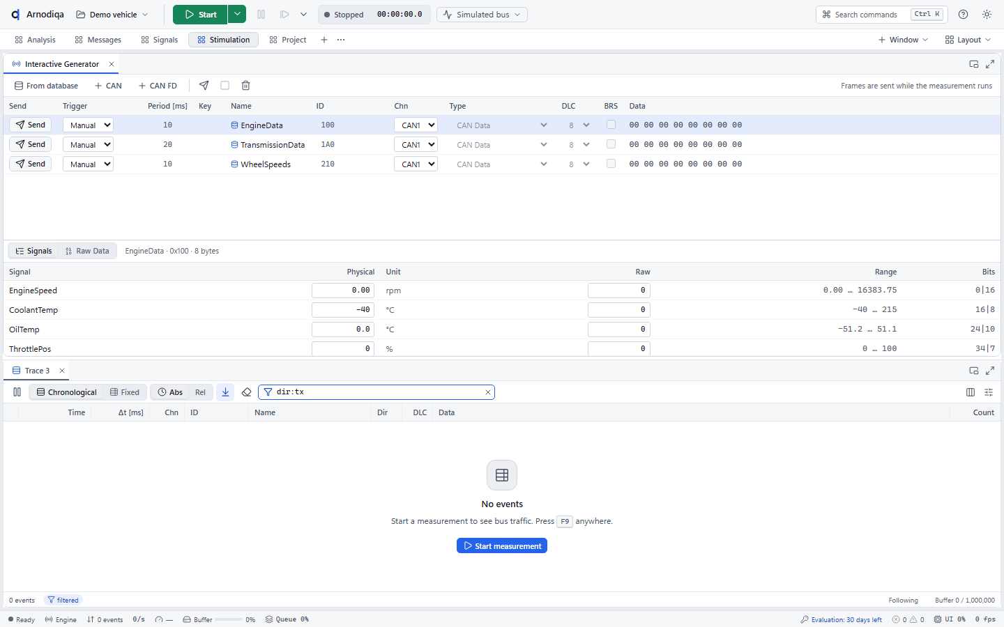
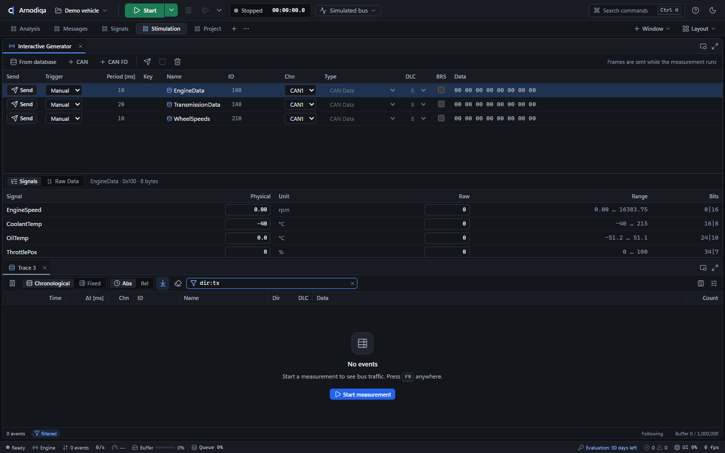
Click + CAN for a custom CAN frame; From database adds a message from the database. Enter the ID (here 7E0) and the data bytes under Raw Data; for a database message, edit the values under Signals.
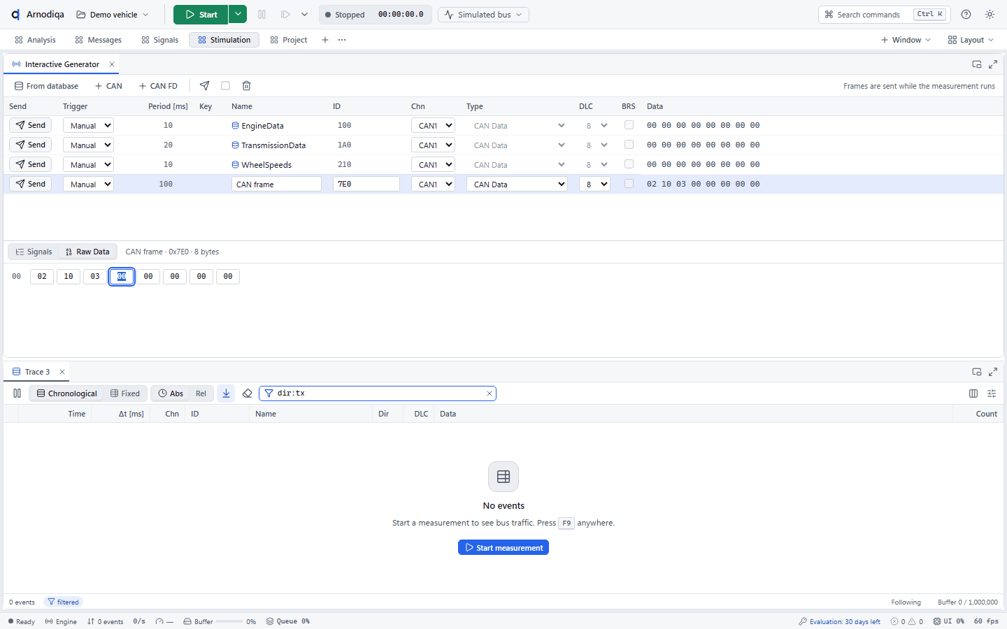
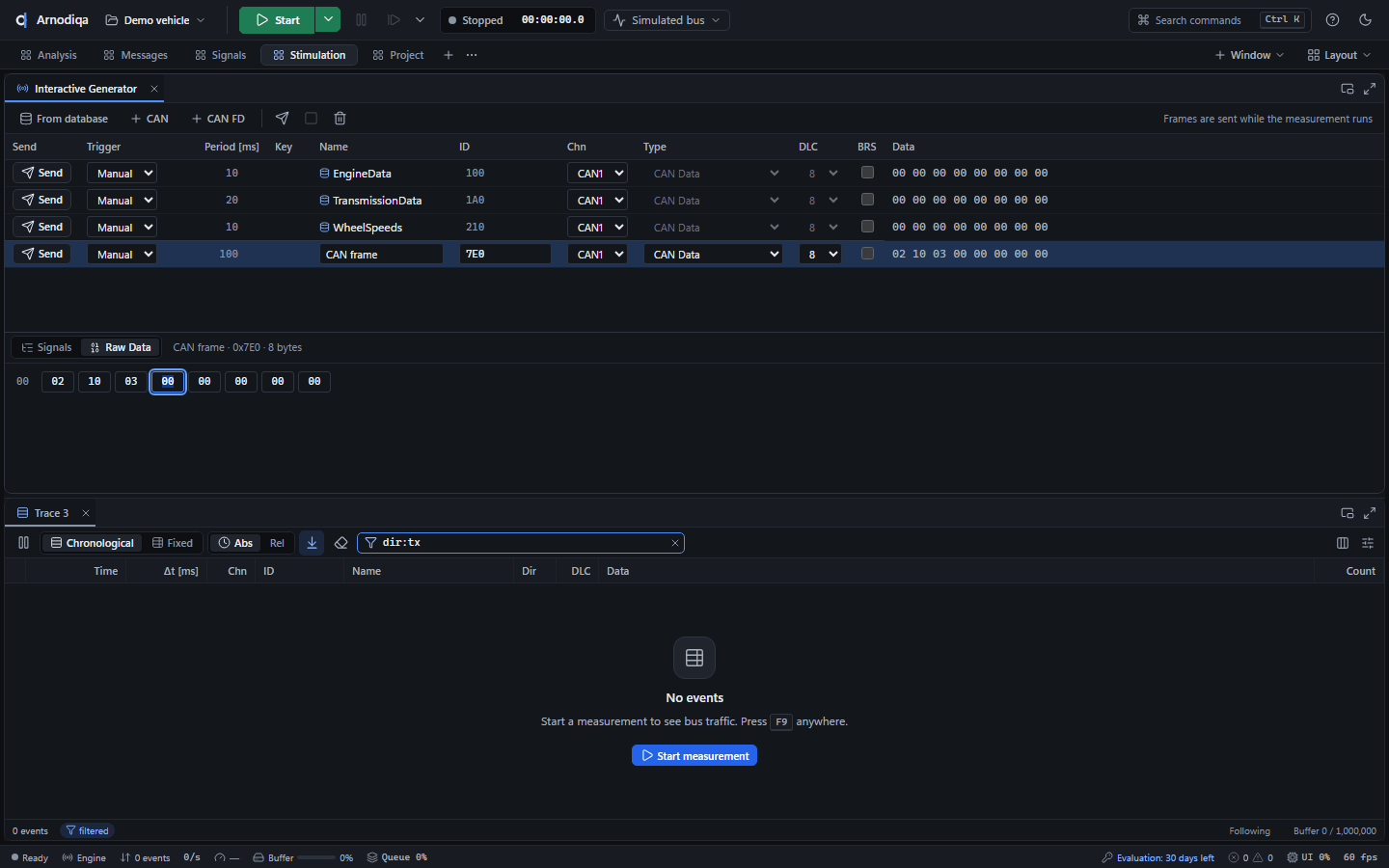
Start the measurement. Send transmits the frame once. Set Trigger to Periodic, enter the period in ms and click Send: the frame is sent cyclically and the button changes to Stop.
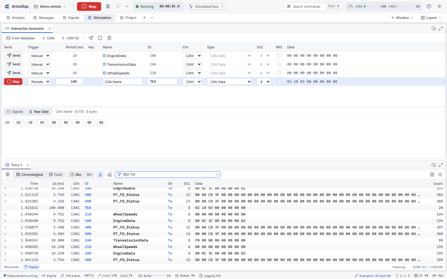
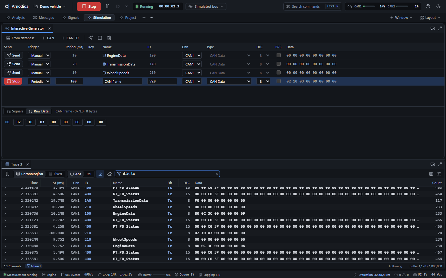
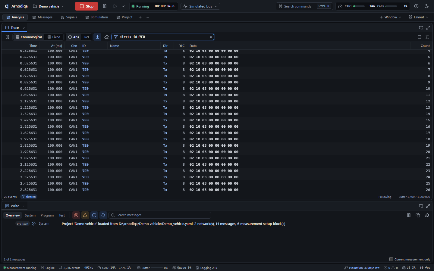
The Trace on the Analysis desktop shows the transmitted frames with direction Tx; the filter
dir:tx id:7E0shows only this frame.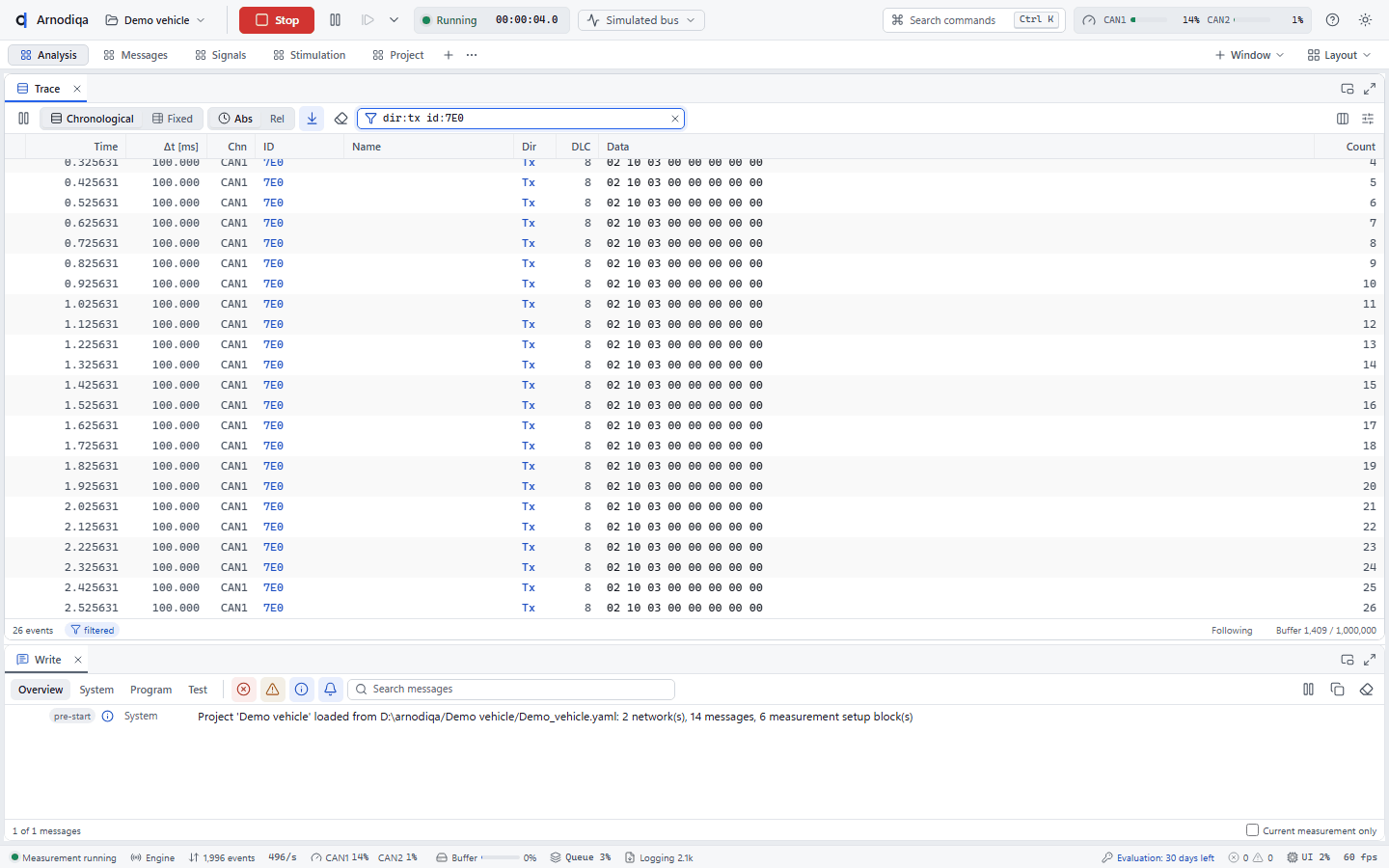
Rest-bus simulation: nodes and interaction layer
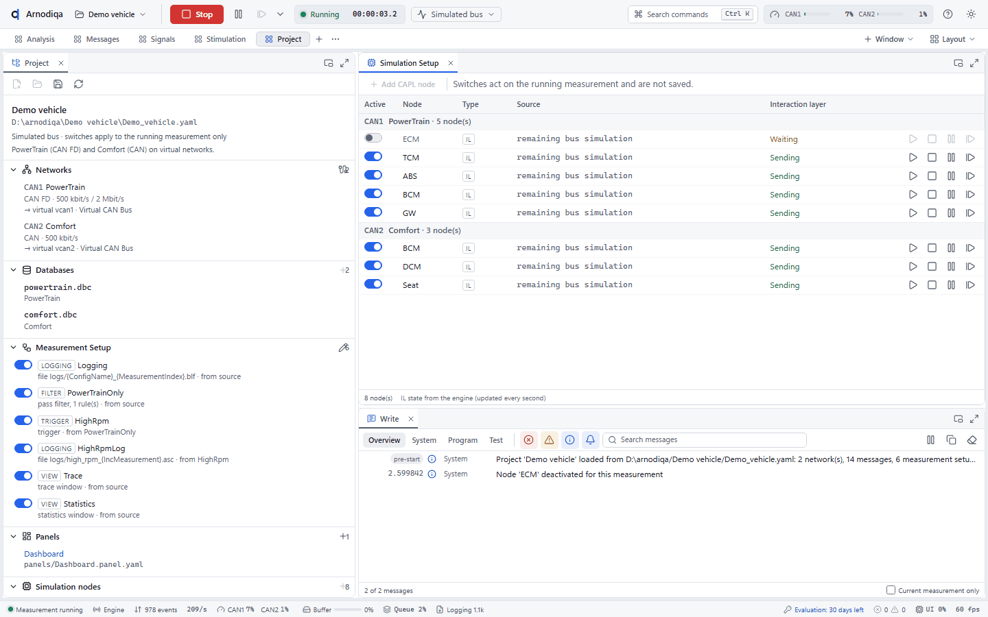
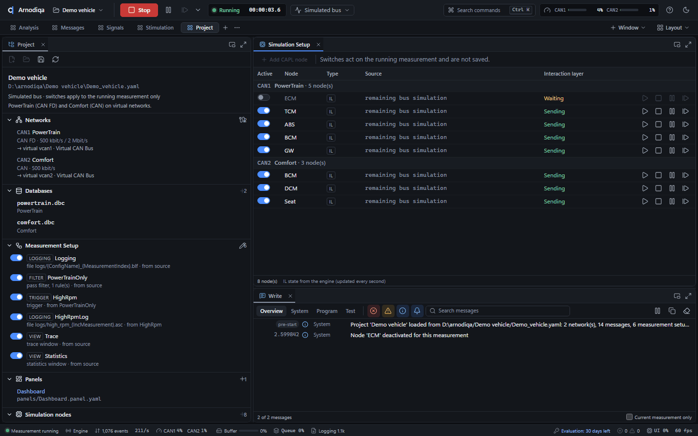
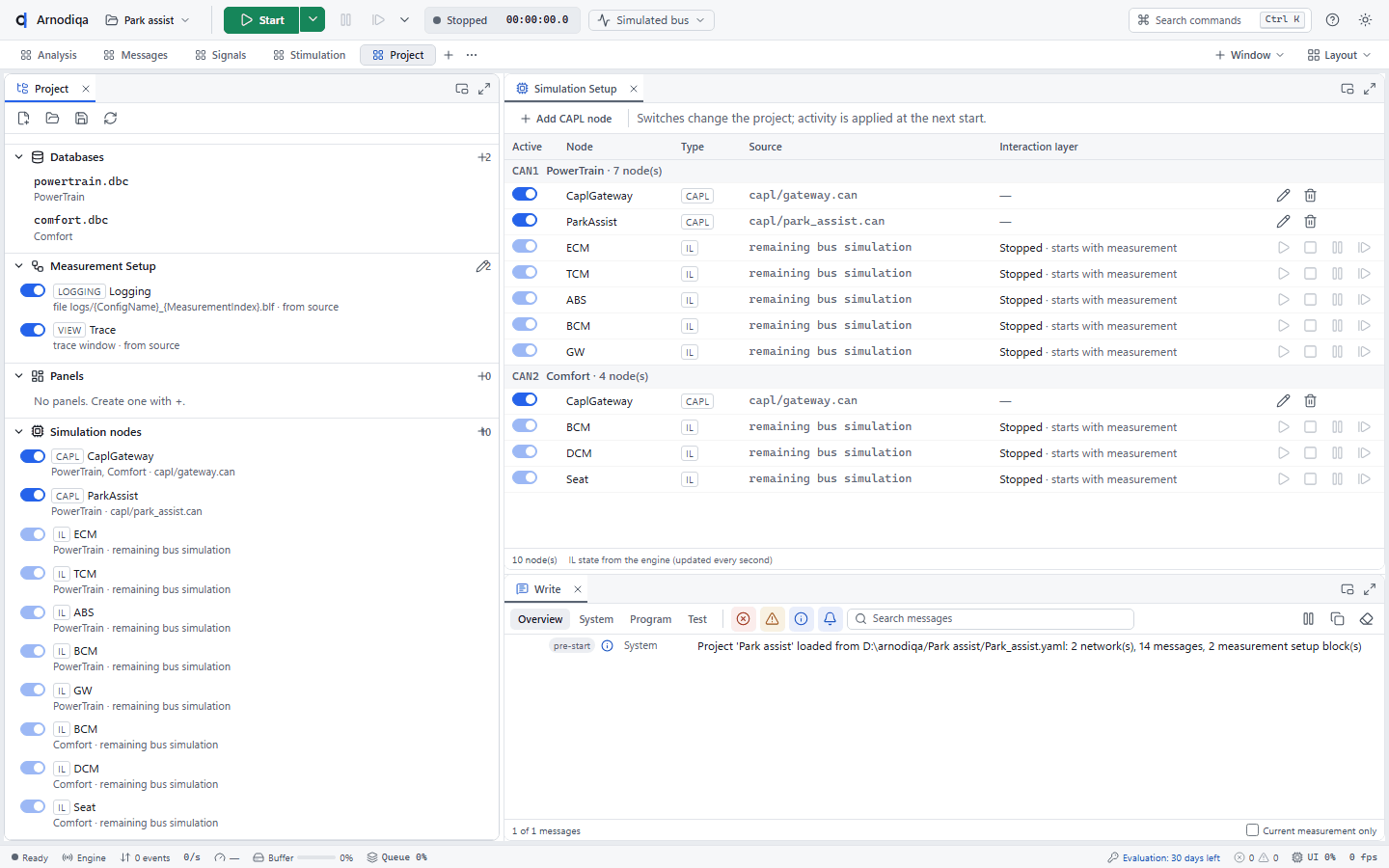
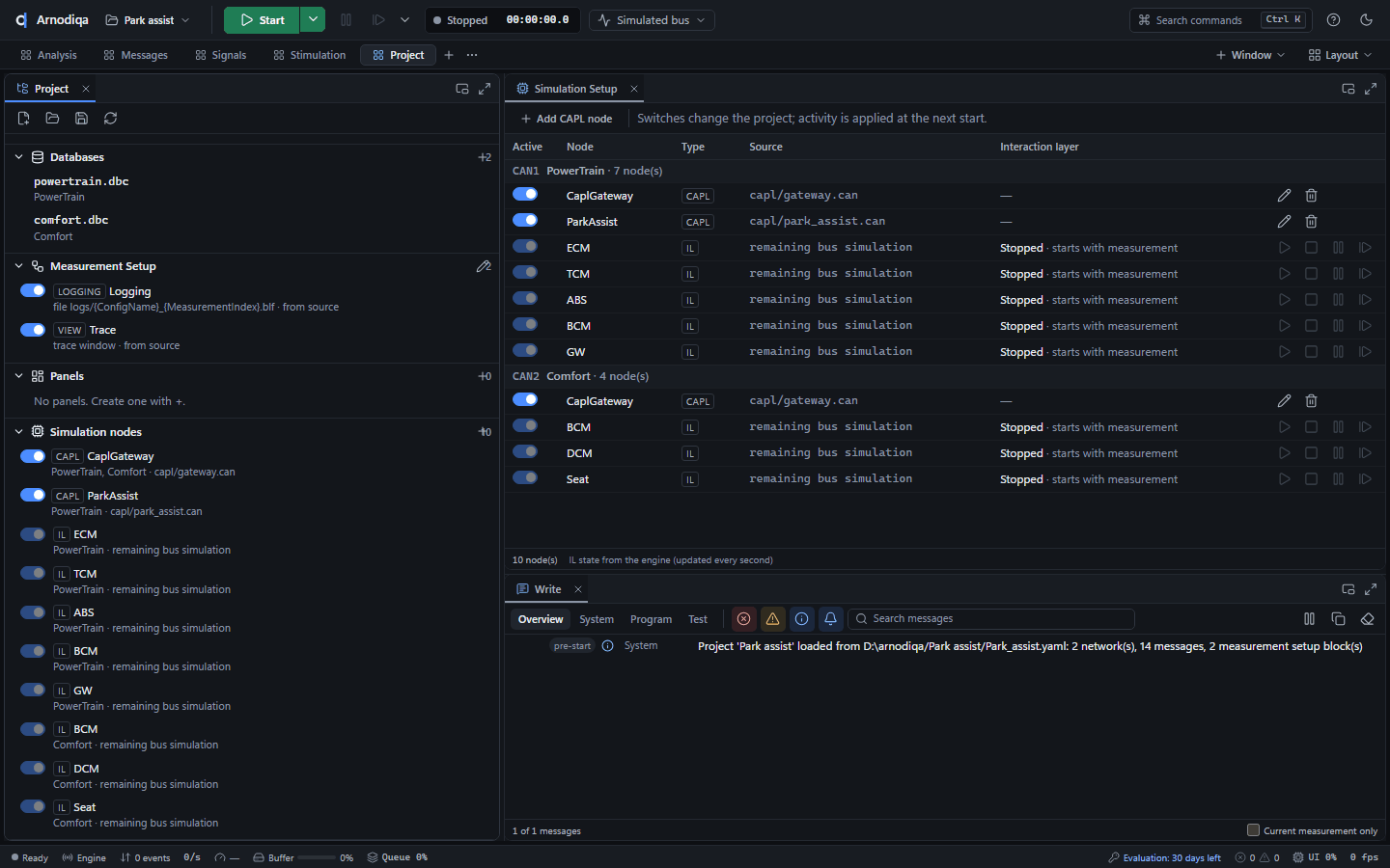
The simulation setup shows the simulated nodes and the state of their interaction layer (IL).
The simulation setup is on the Project desktop, or open it with Ctrl+K and New Simulation Setup window. For each network you see the nodes with type (IL = interaction layer), source and the state of the interaction layer.
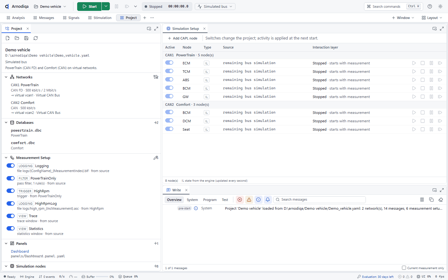
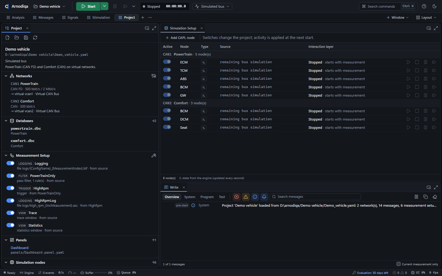
Start the measurement: the IL nodes send their messages according to the database (Sending).
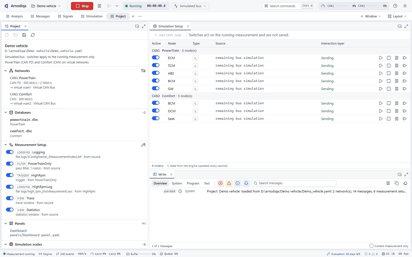
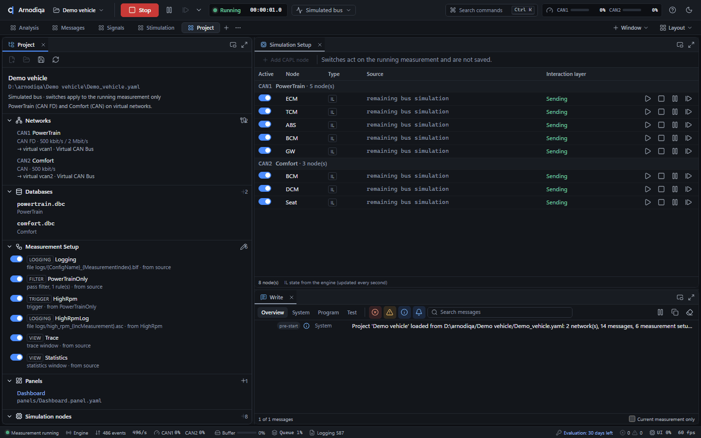
Use Stop IL and Start IL at the right of the row to stop or restart the interaction layer of one node while the measurement continues.
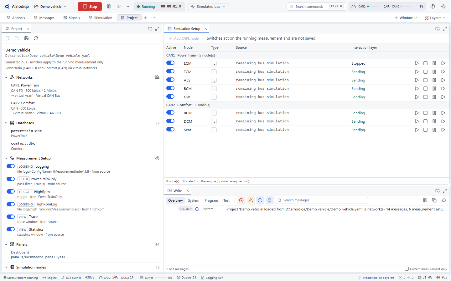
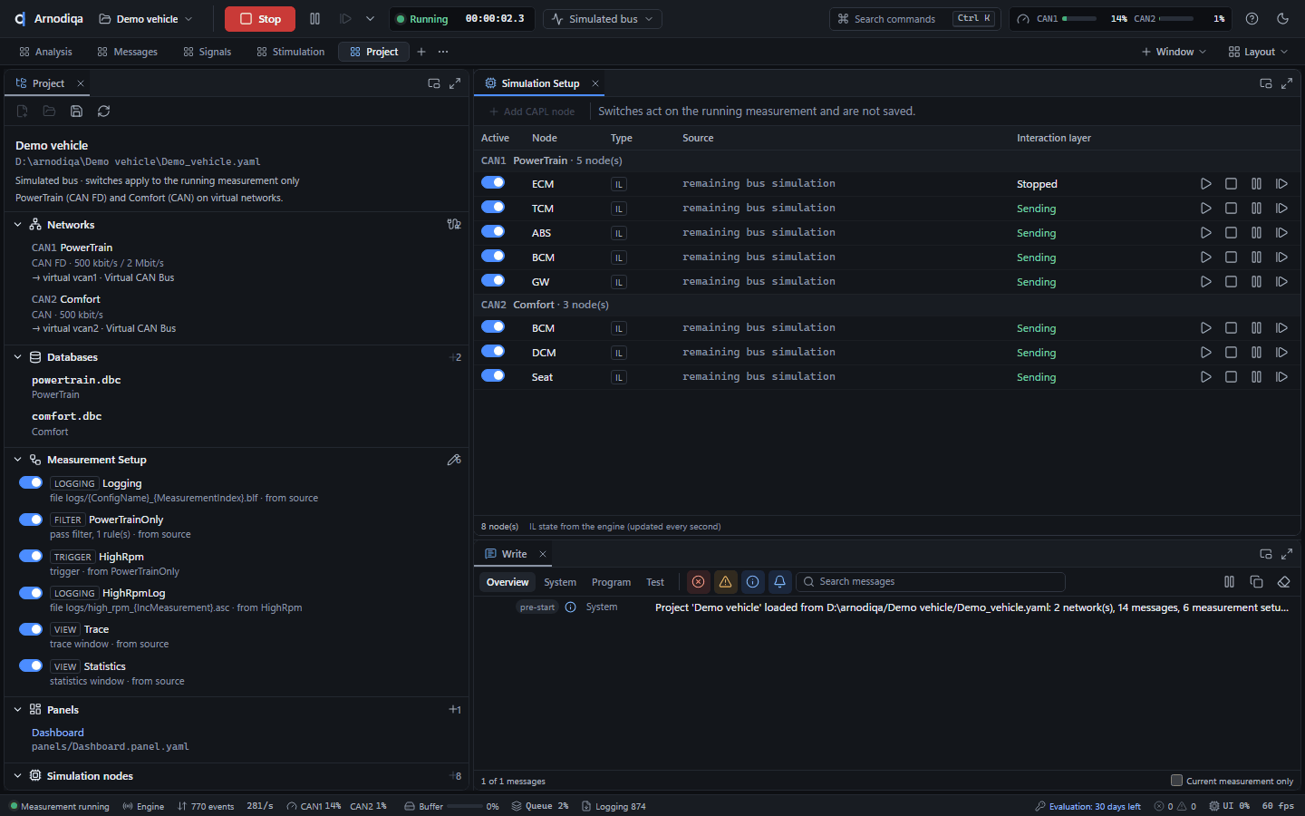
The switch in the Active column turns a node off completely, for example to let a real ECU transmit in its place. During a measurement this applies to that measurement only; when stopped, the switch changes the project.
Record, replay offline and replay blocks
Logging blocks in the measurement setup write BLF, ASC, MF4 or PCAPNG. A recording is replayed offline through the same analysis as a live measurement, or put back on the bus with a replay block.
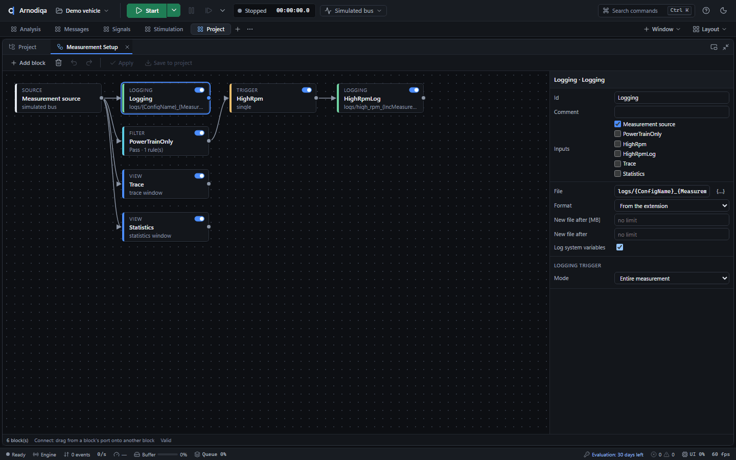
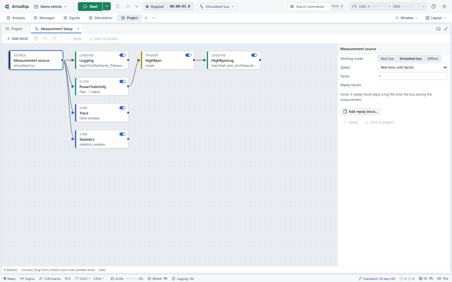
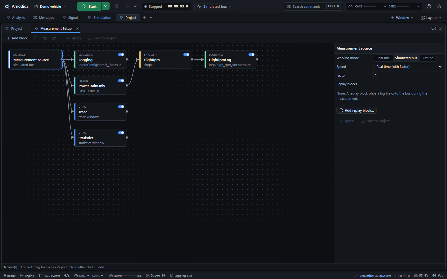
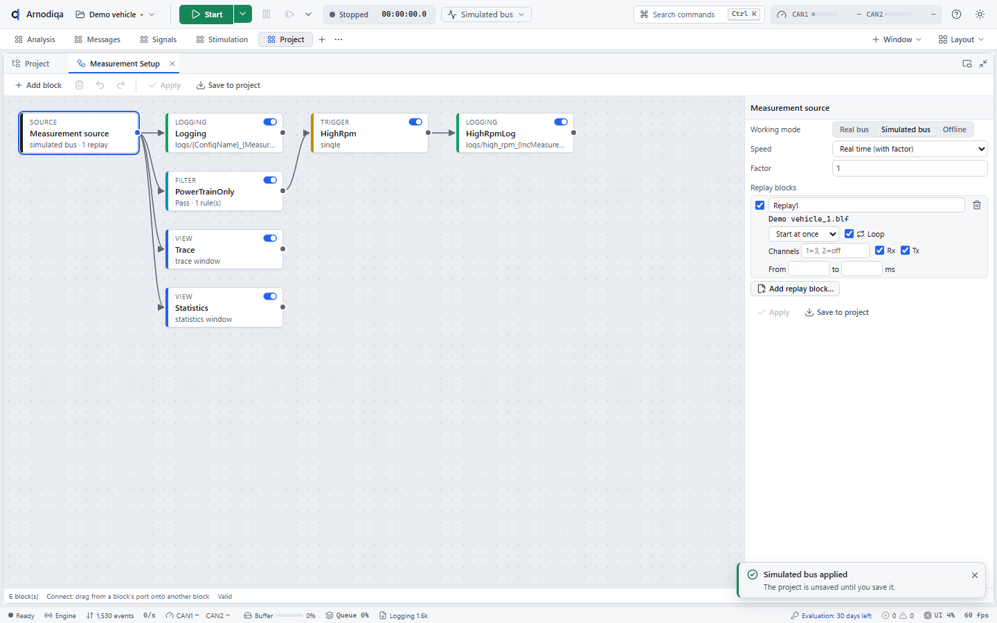
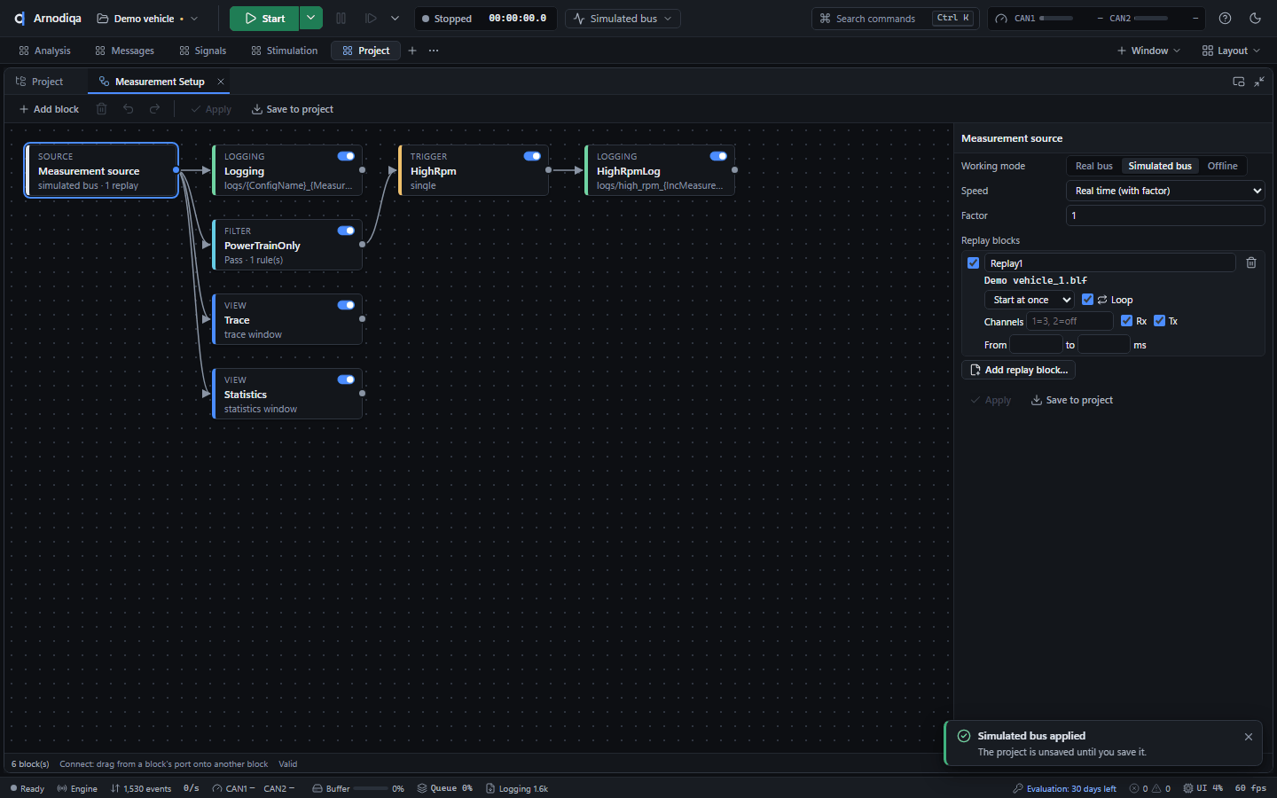
In the project explorer, click the pencil next to Measurement Setup. The editor shows the graph from Measurement source to filters, triggers, logging and windows. For a logging block, the right side shows File (with field codes such as {MeasurementIndex}, button
{…}), Format, New file after [MB] and the Logging trigger. Add block adds a block; Apply and Save to project keep the change.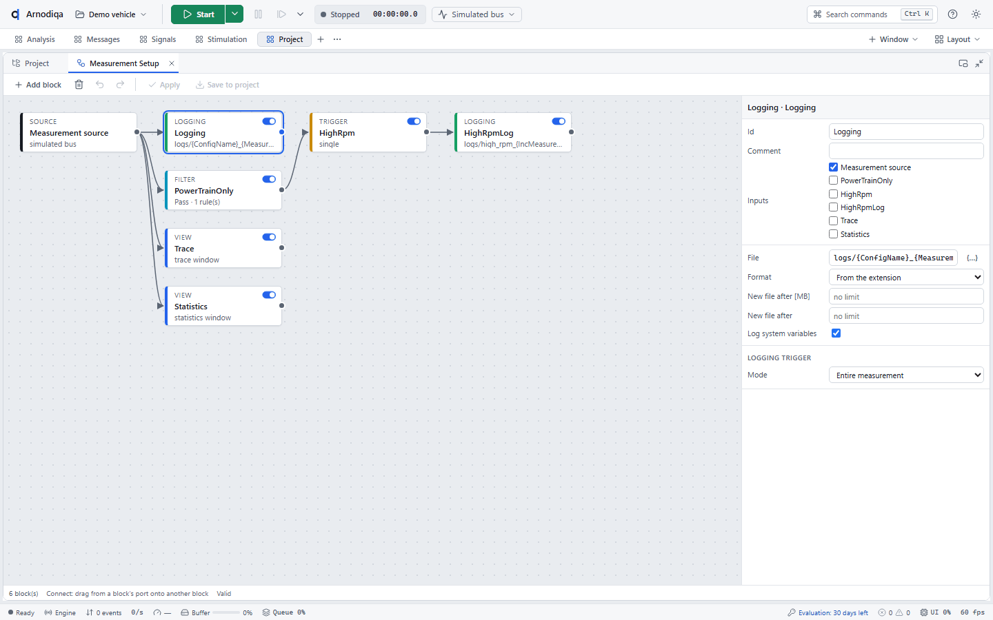
Start and stop the measurement. Each enabled logging block writes its file in the project folder, here logs/Demo vehicle_1.blf and, for the trigger block HighRpm, logs/high_rpm_001.asc. During the measurement the status bar shows Logging with the number of events. The switch next to a block in the project explorer turns logging on or off; Start measurement without logging skips logging once.
In the measurement setup, click the Measurement source block. On the right, choose the working mode: Real bus (the networks' hardware), Simulated bus (all networks simulated, virtual time) or Offline (replay log files). The replay blocks are listed below.
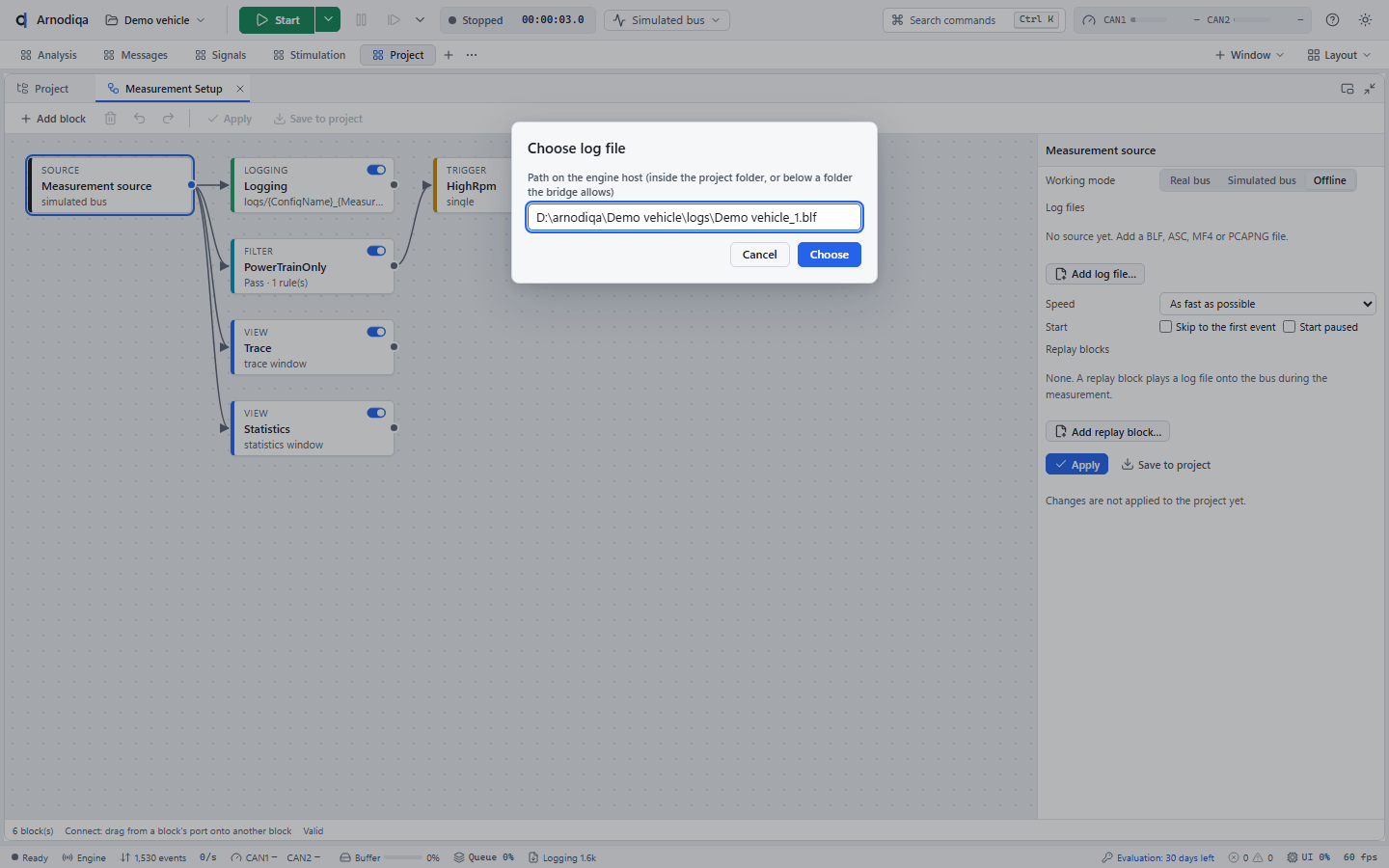
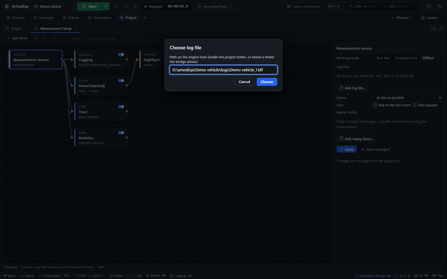
Choose Offline, click Add log file… and select one or more BLF, ASC, MF4 or PCAPNG files, here the recording from step 2.
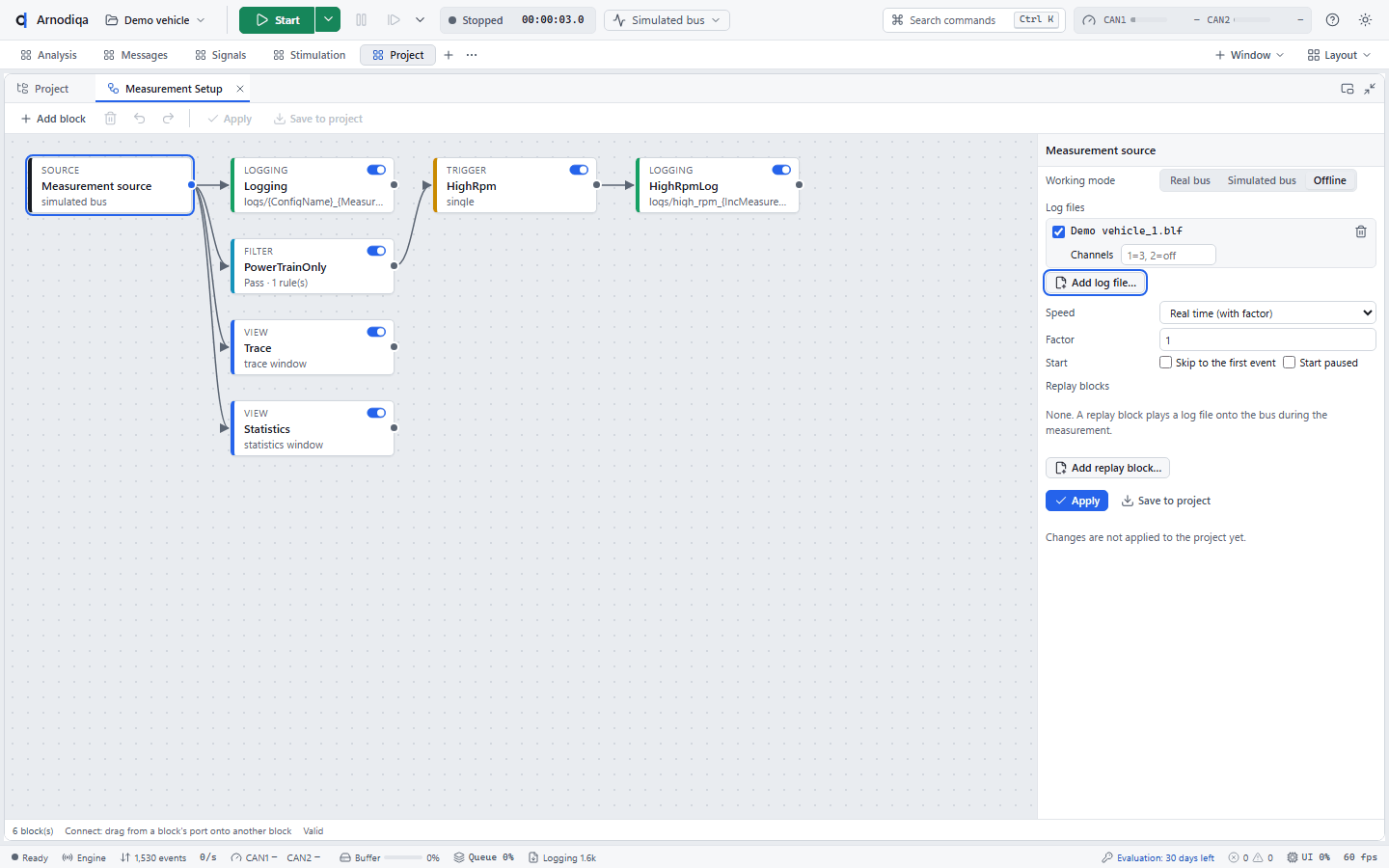
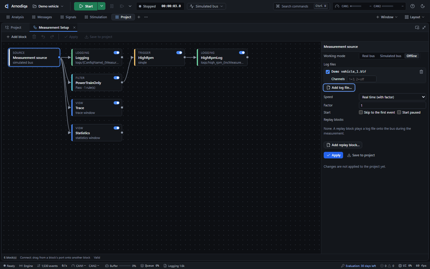
The log file is listed under Log files; the tick disables a source temporarily, the bin removes it. Under Speed, choose As fast as possible, Real time (with factor) (2 = half speed) or Animate (one event per delay). With several files, Order determines how they are merged; Skip to the first event and Start paused are under Start.
Click Save to project (Apply applies the change without saving). The toolbar now shows Offline and the source block offline · 1 file. The same is available via Ctrl+K with Working mode: Offline (log files).
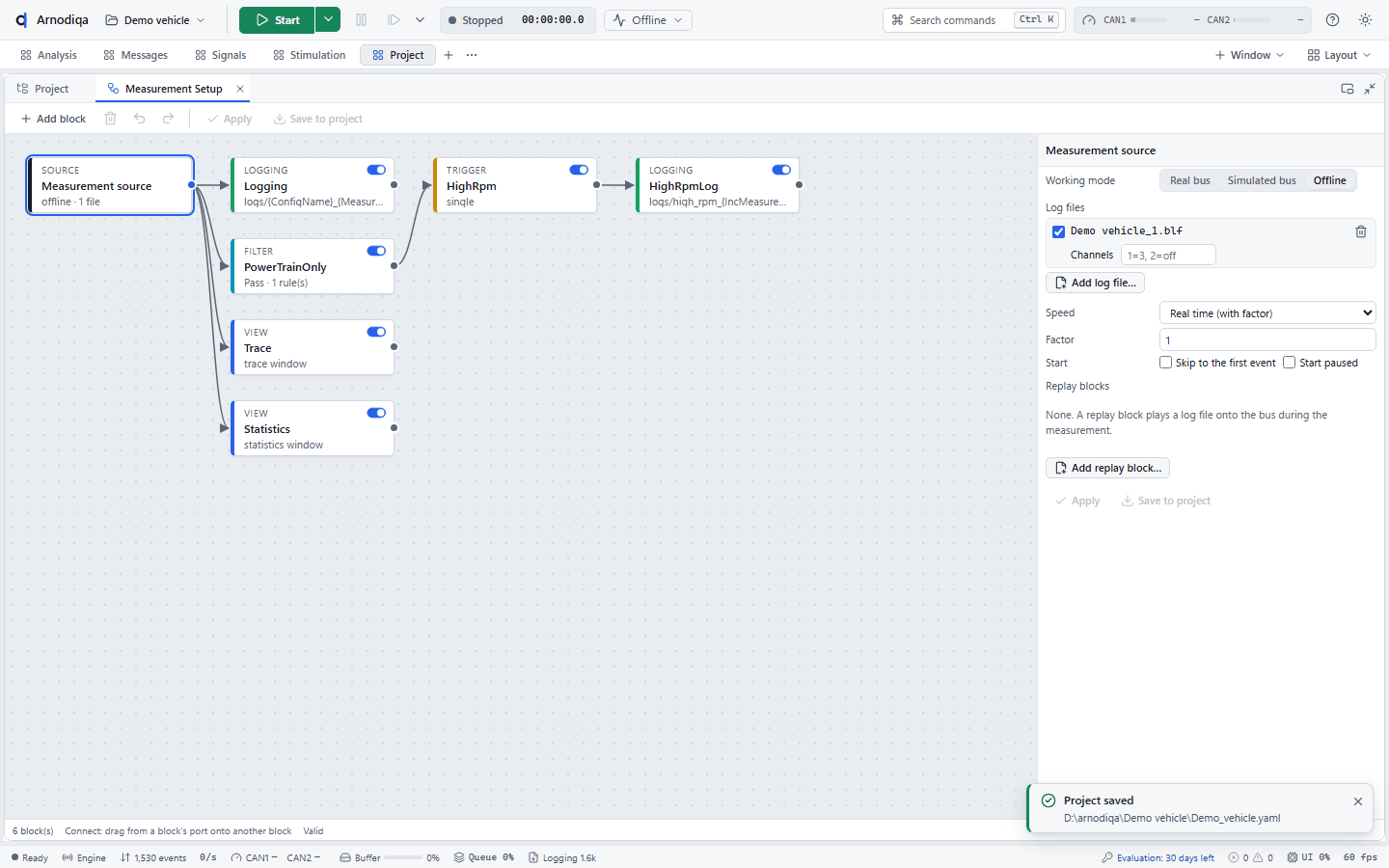
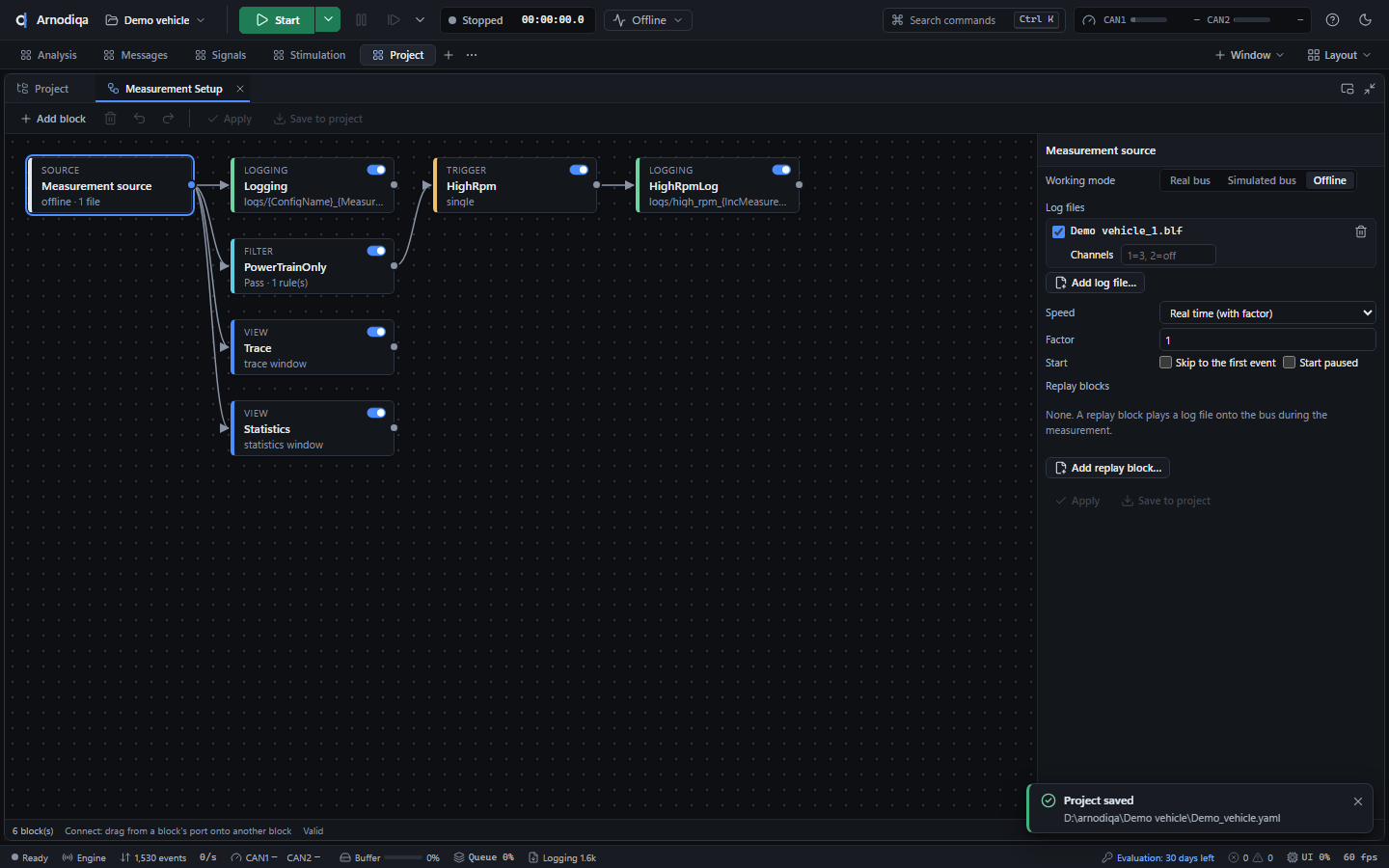
Click Start (F9): Arnodiqa replays the log file through the same analysis as a live measurement (Trace, Graphics, Statistics). At the end of the file the measurement stops automatically; with Real time this takes as long as the recording.
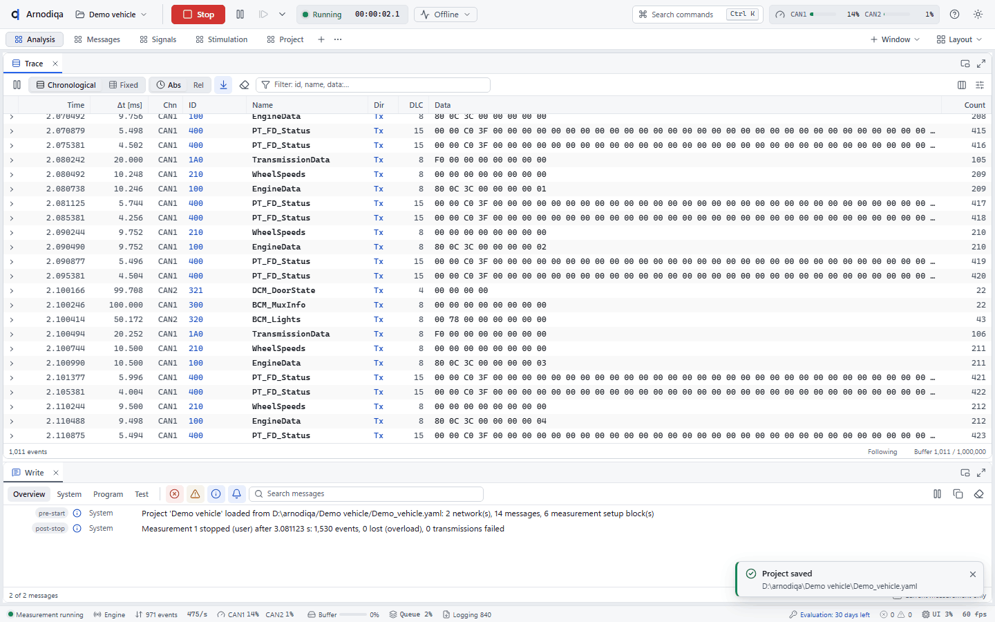
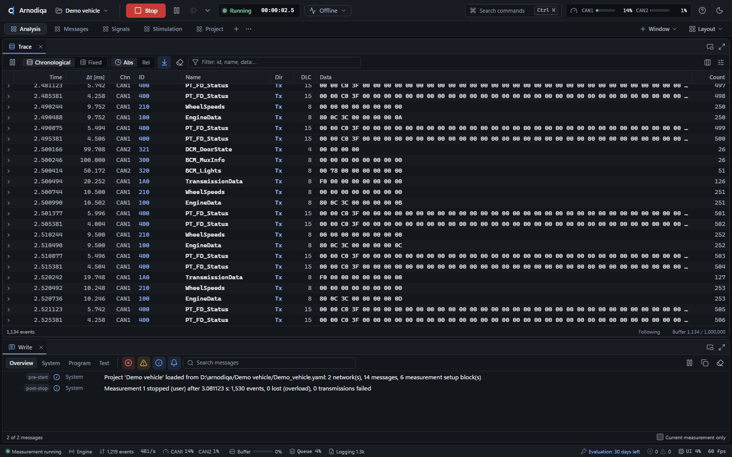
To put a recording back on the bus during an online measurement, choose Simulated bus or Real bus and click Add replay block… under Replay blocks. For each block, choose the name, Start at once, Original times or Delayed, and Loop. Apply puts the block in the project. At the next start the block sends the frames from the file. In offline mode, replay blocks are inactive.
Diagnostics: UDS console and fault memory
Diagnostic Console and Fault Memory work with the project's diagnostic ECUs, simulated or real.
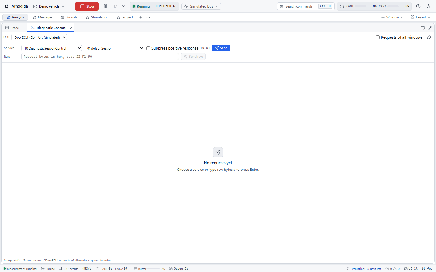
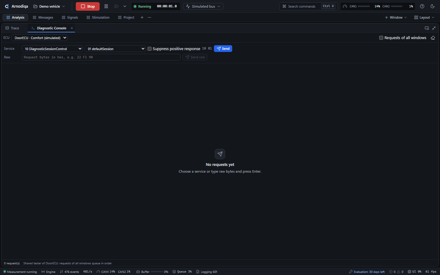
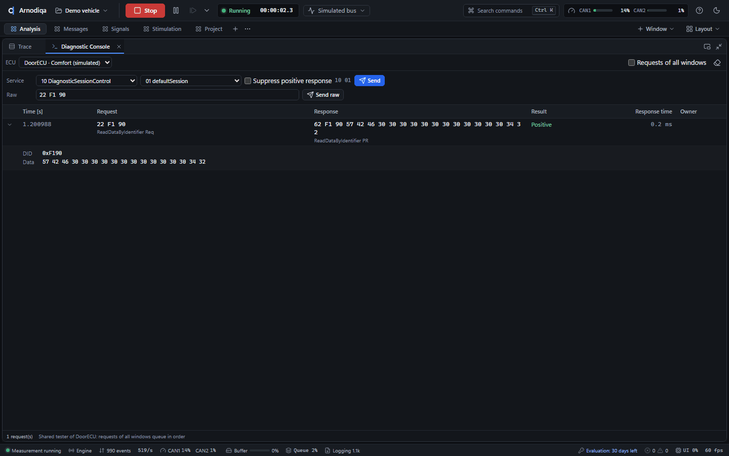
Open the Diagnostic Console with Ctrl+K and New Diagnostic Console window and start the measurement. Select the ECU under ECU (here DoorECU). Choose a service and subfunction under Service and click Send, or type a request in hex under Raw.
Type for example
22 F1 90(ReadDataByIdentifier, VIN) under Raw and press Enter or click Send raw. The history shows request, response, result and response time; click a row for the decoded parameters. A negative response shows the NRC with its name.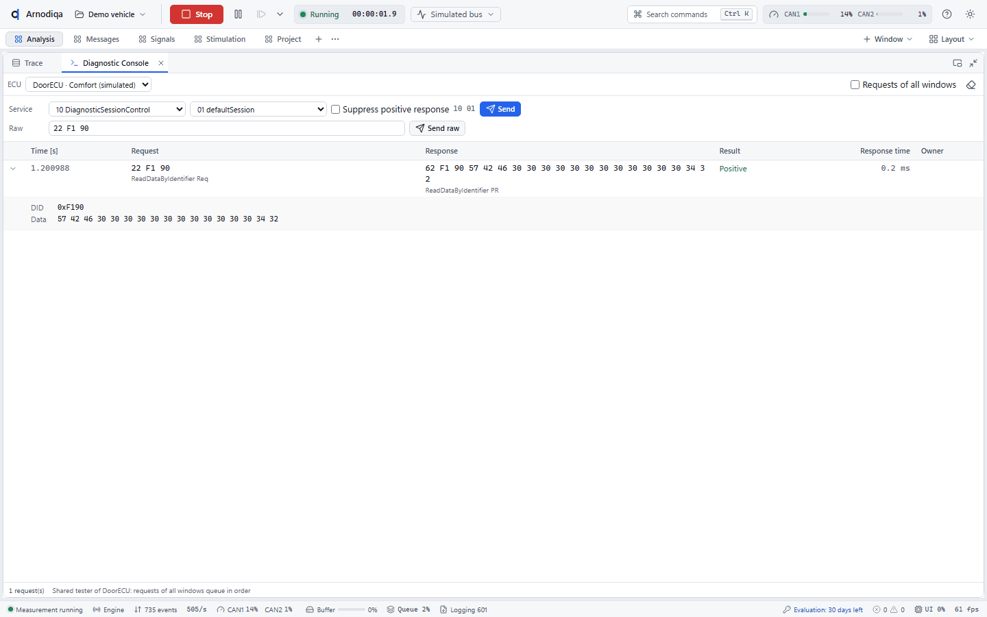
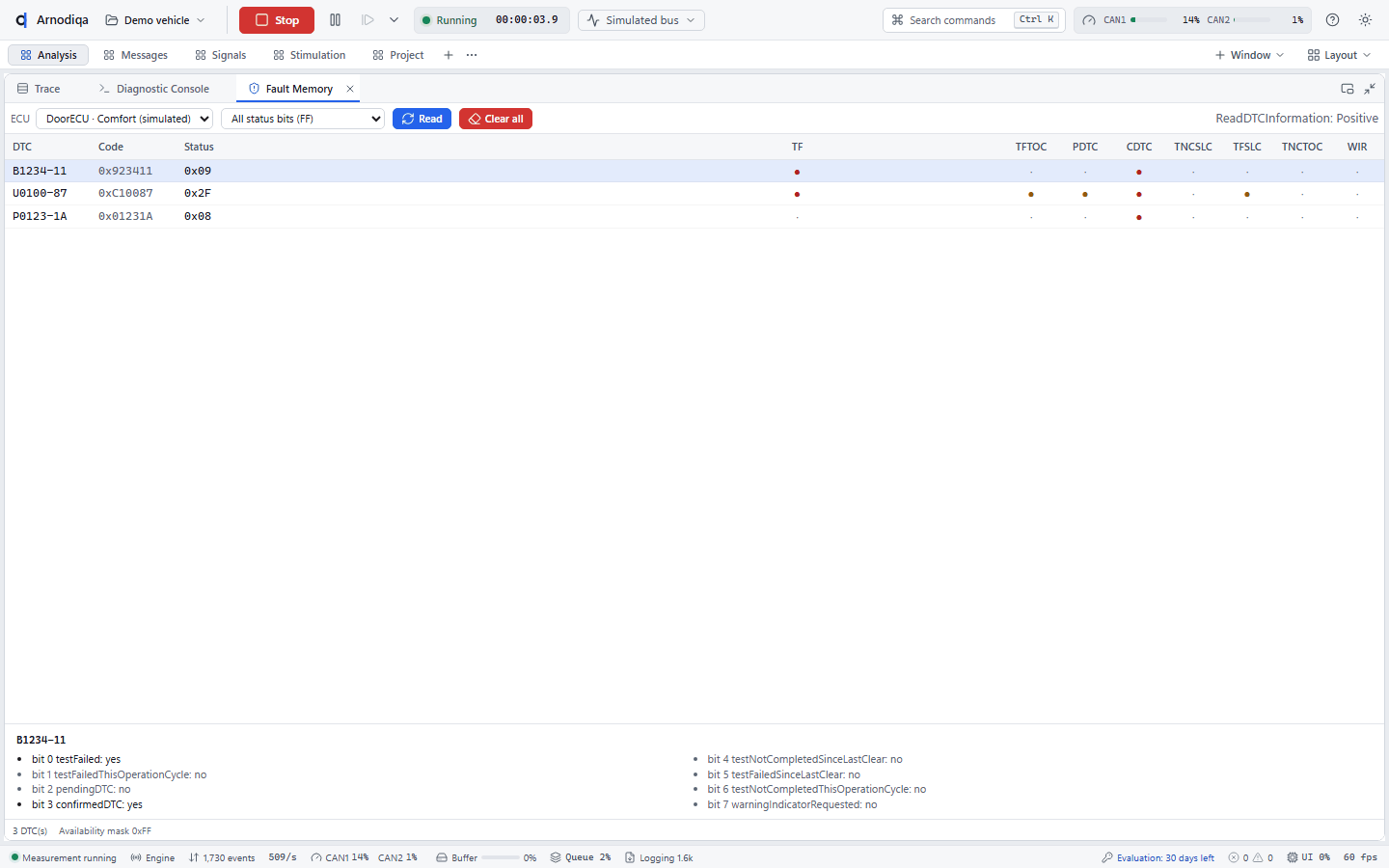
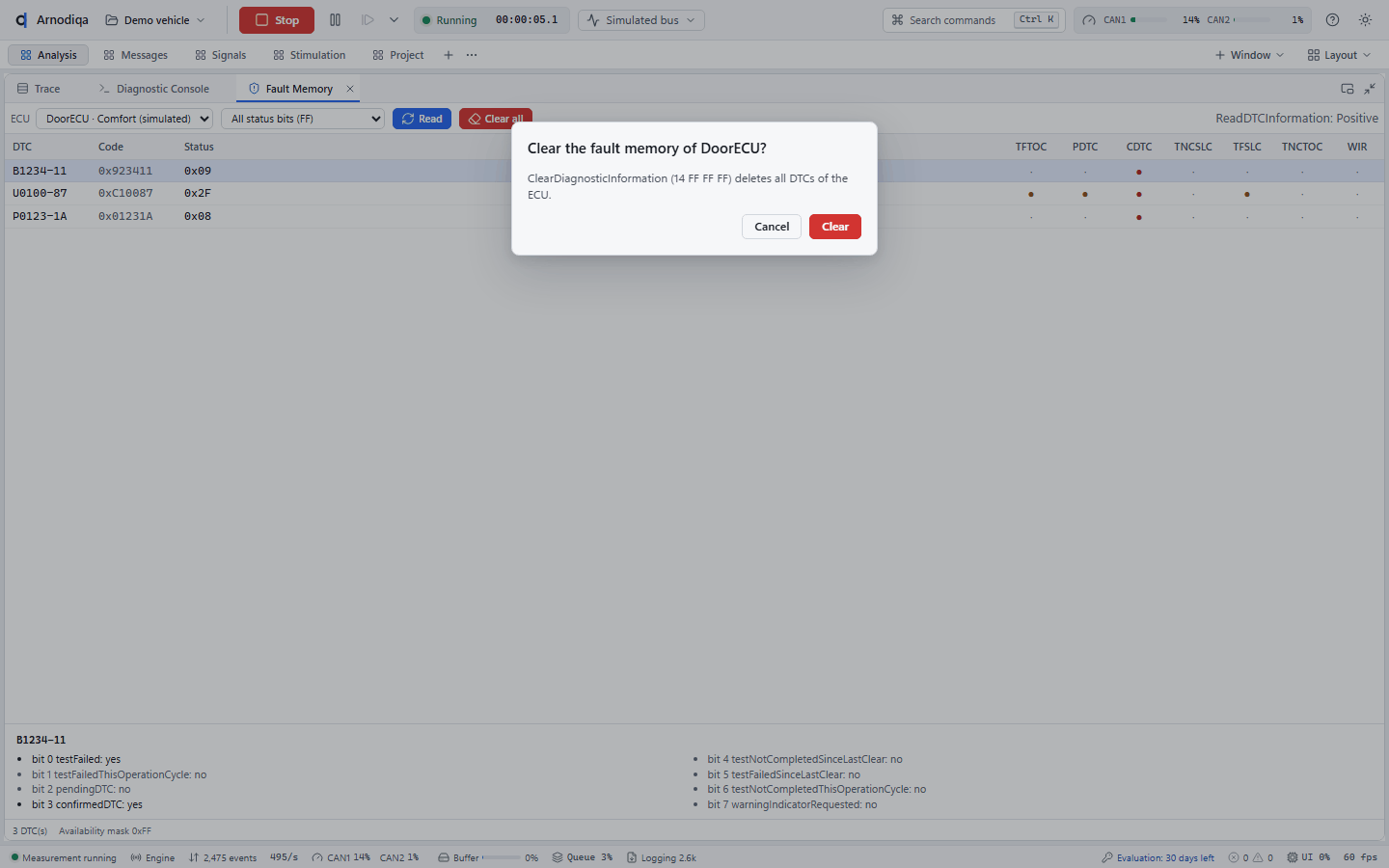
Open Fault Memory (Ctrl+K, New Fault Memory window) and click Read (service 19 02 with the status mask from the list, default All status bits (FF)). For each DTC you see the SAE code, code, status and the status bits as columns; at the bottom the eight bits of the selected DTC are written out.
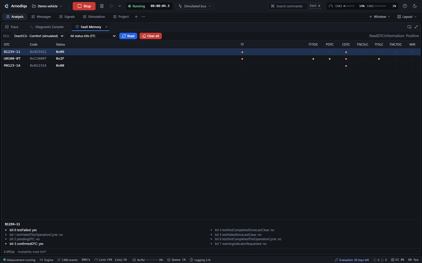
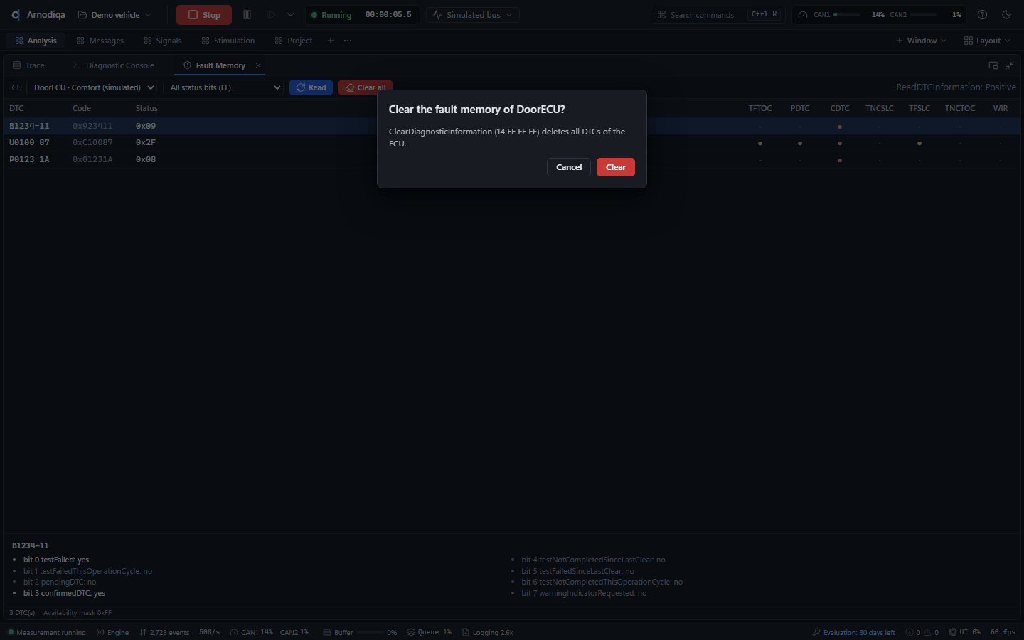
Clear all clears the fault memory (ClearDiagnosticInformation, 14 FF FF FF); confirm with Clear.
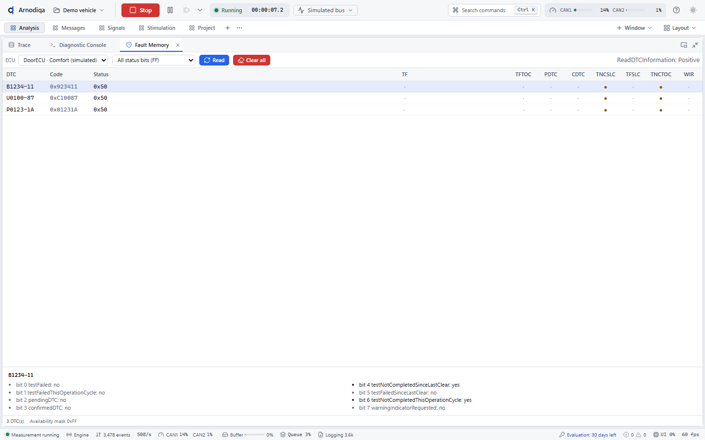
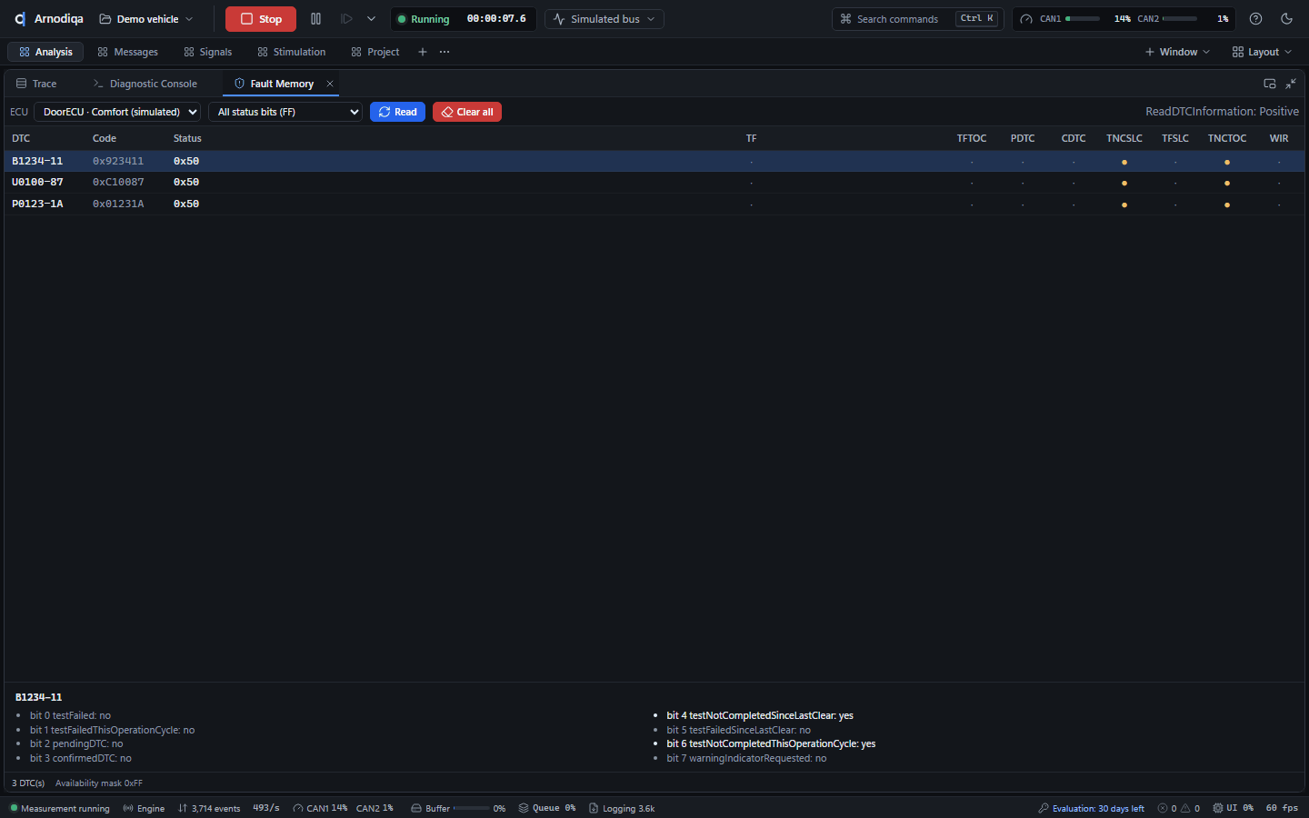
After clearing, Read reads the DTCs again: their status has been reset.
Flash an ECU
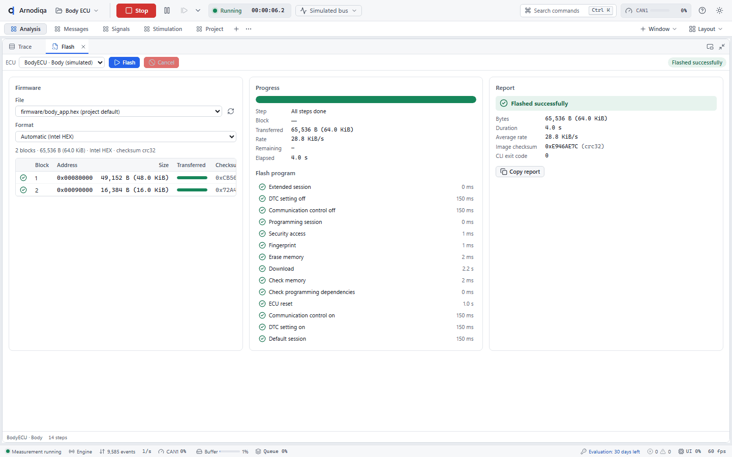
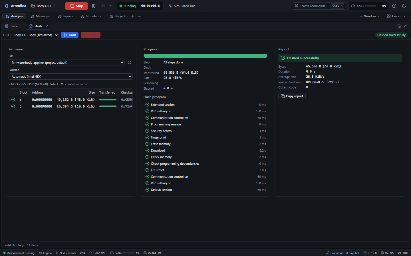
The Flash window runs an ECU's flash program, with progress per step and per block.
Open the Flash window (Ctrl+K, New Flash window) and start the measurement. Choose the ECU, the firmware file (by default the one from the project, or via Browse…) and the format. The window shows the blocks of the file in advance.
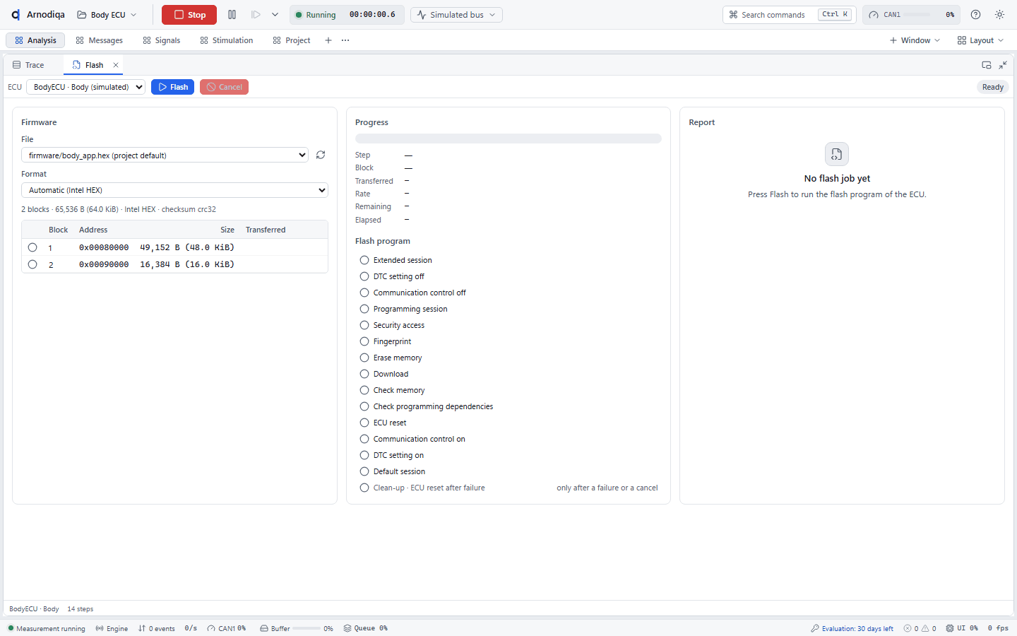
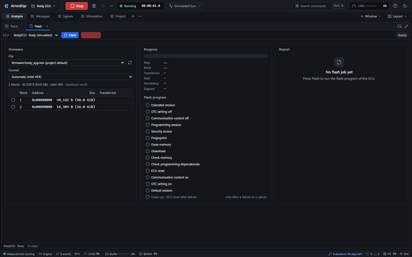
Click Flash (Ctrl+Enter). The progress bar, current step, block, rate and remaining time are updated. Cancel aborts; the clean-up steps still run.
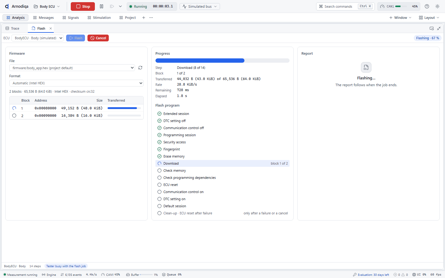
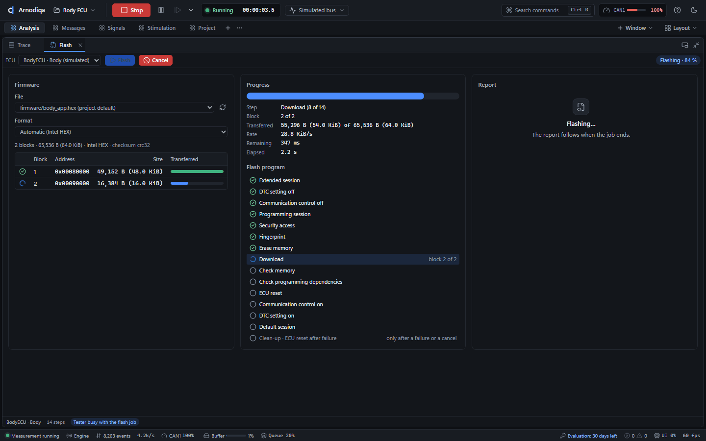
The final report shows the outcome, duration, rate and checksums. Copy report copies the report; on a failure it includes the failing step and the NRC.
Add and edit CAPL nodes
Existing CAPL programs run as simulation nodes alongside the rest-bus simulation. The built-in CAPL Editor checks the program while you type.
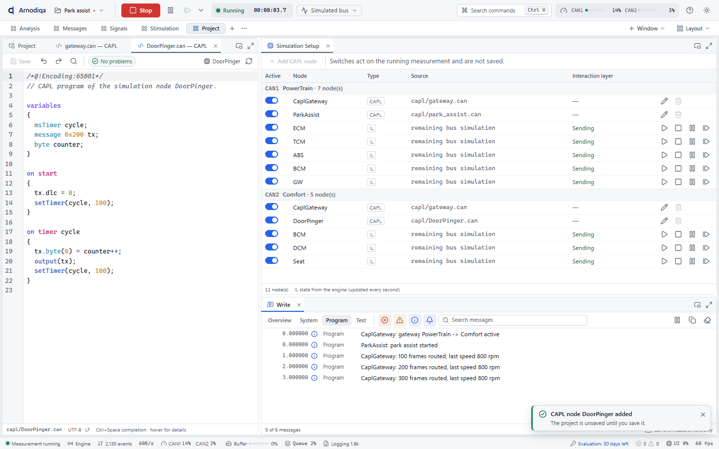
On the Project desktop, the CAPL nodes are listed under Simulation nodes with their source file (.can) and networks. In the simulation setup their type is CAPL; the pencil opens the program in the CAPL Editor, the bin removes the node from the project and Add CAPL node adds one.
The CAPL Editor shows the program with syntax highlighting and line numbers. At the top right are the nodes that run this file (here CaplGateway); No problems comes from the same compiler as at measurement start and in
arnodiqa capl check.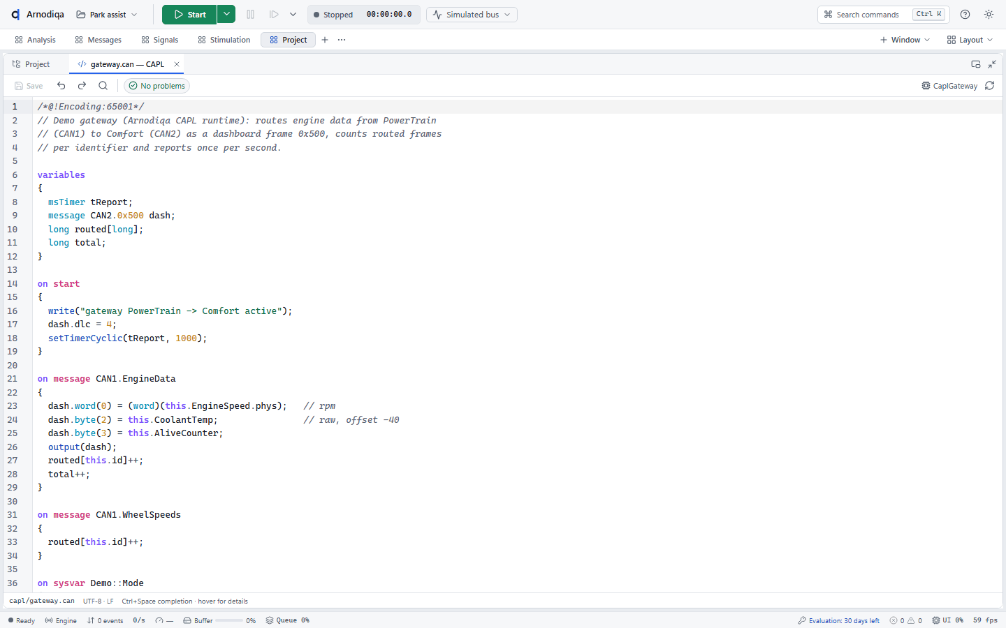
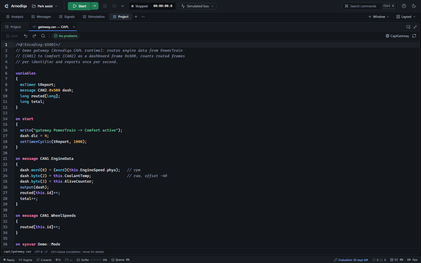
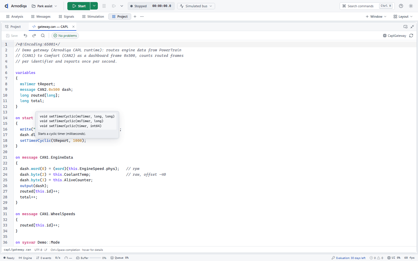
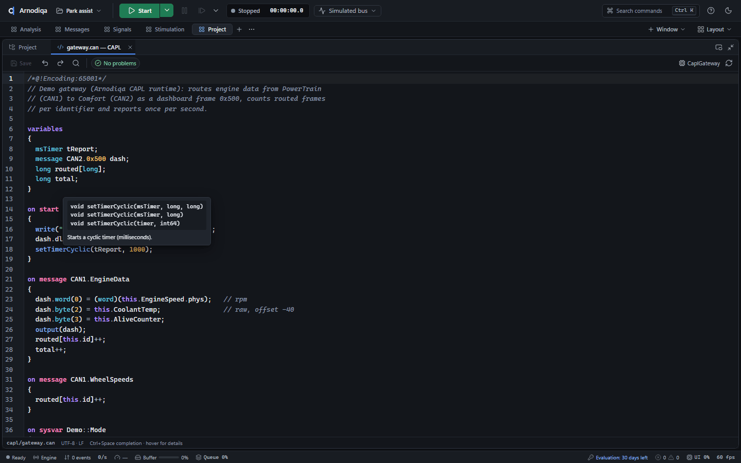
Hover over a name for details: for a CAPL function all its forms with their parameters, for a message the ID, length, cycle time and signals, for a signal the scaling, unit and value table.
Arnodiqa checks the program while you type: errors get a red wavy underline and a marker in the margin, and the counter in the toolbar shows the number of errors and warnings (click it for the list, or Ctrl+Shift+M). Here totl is unknown and a semicolon is missing.
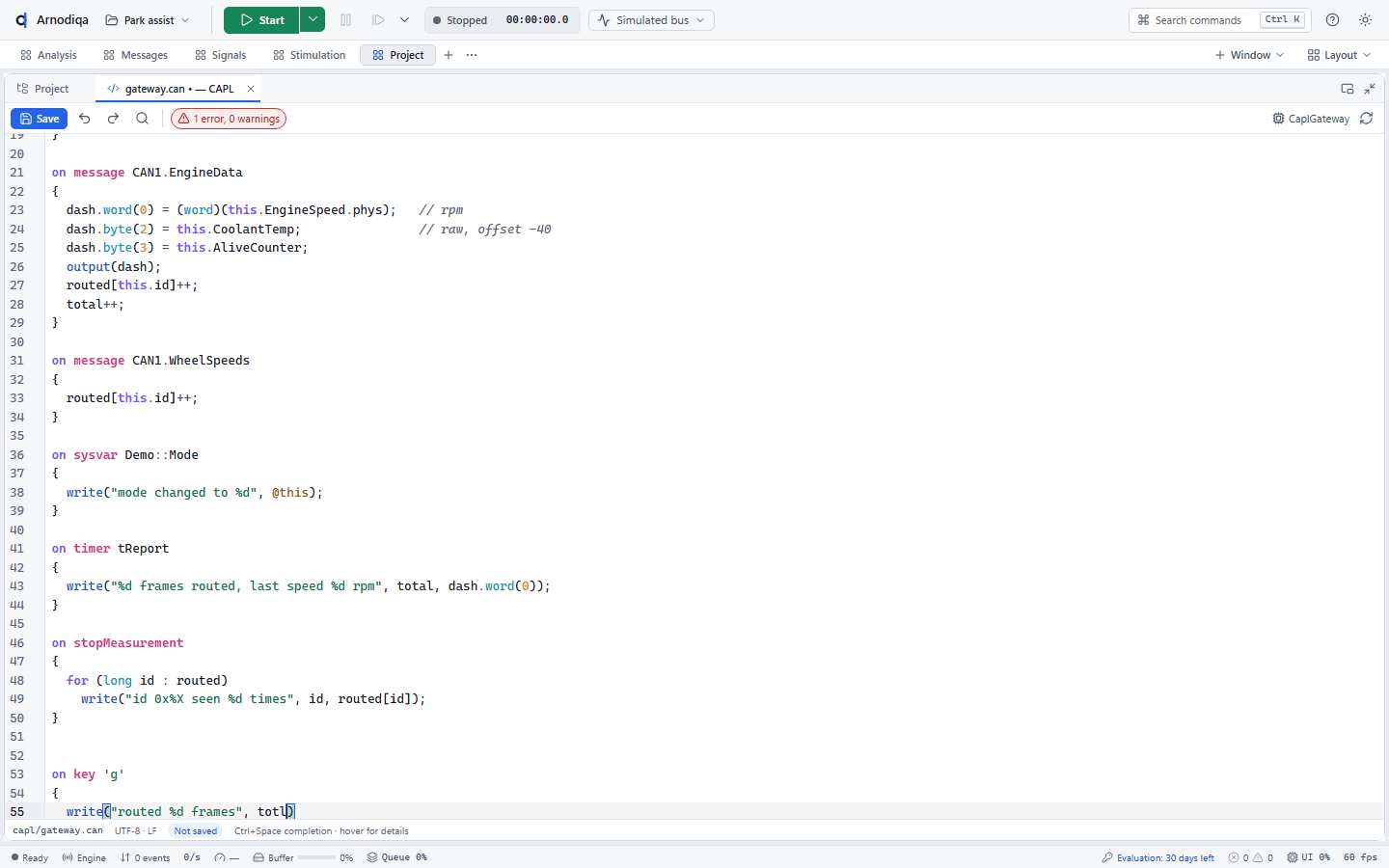
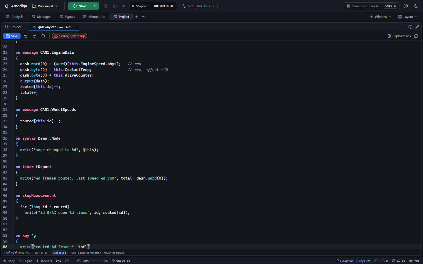
Ctrl+Space, or simply typing, shows completions: variables, functions and CAPL functions, messages and signals from the project's databases, and after @ the system variables. Enter or Tab accepts the choice.
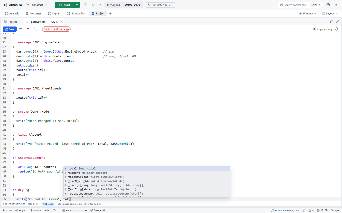
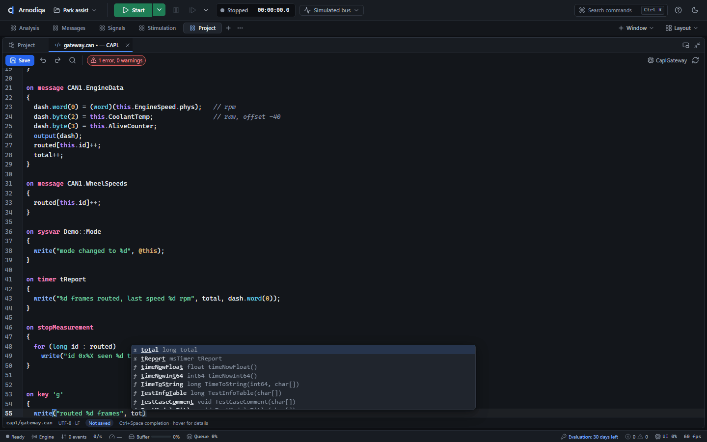
Ctrl+S (or Save) saves the file and reloads the node with the new program. During a measurement Arnodiqa asks for confirmation first; the running measurement keeps the old program until the next start.
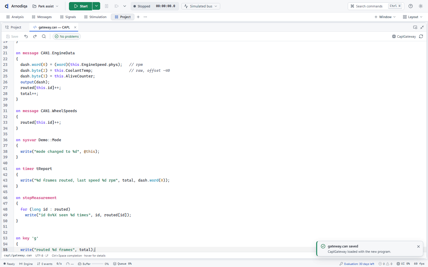
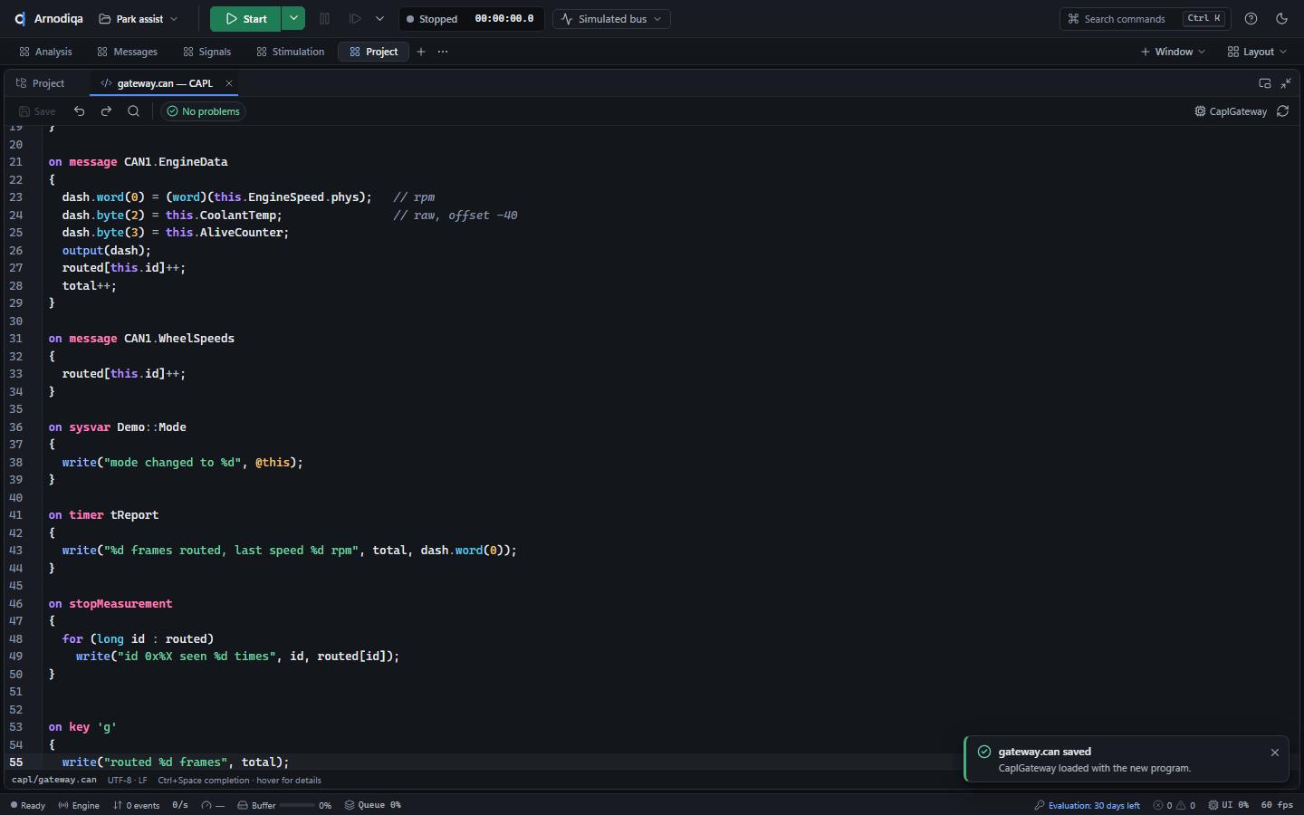
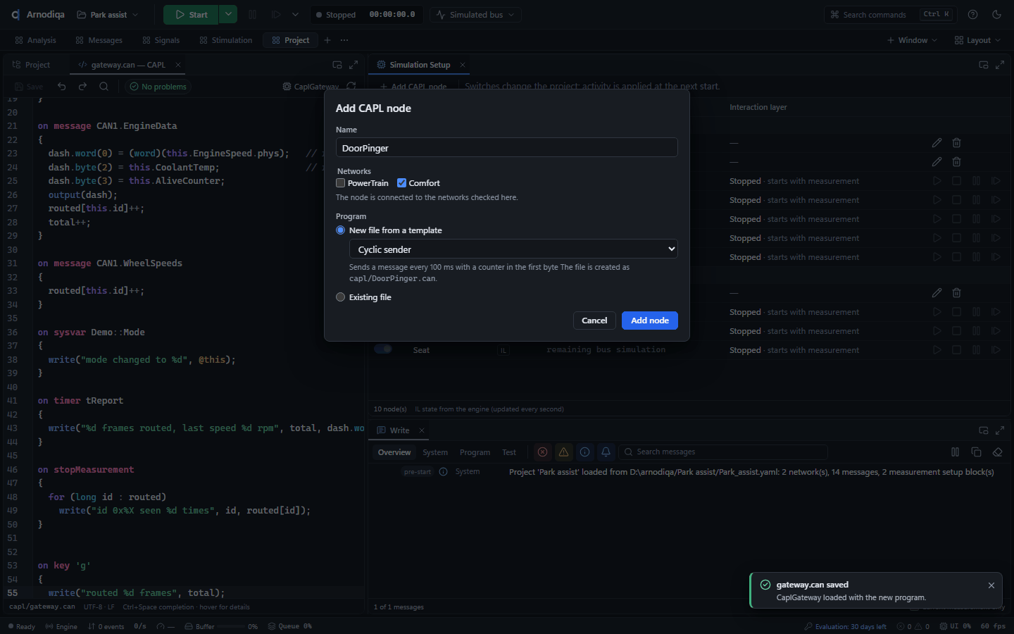
To add a node, click Add CAPL node in the simulation setup or the + next to Simulation nodes in the project explorer. Enter a name, choose the networks and a template (Empty node, Cyclic sender, Echo / gateway); the file becomes capl/<name>.can. Existing file uses an existing .can file, inside the project folder or outside it (copied or referenced with a relative path).
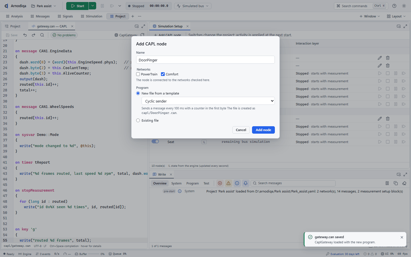
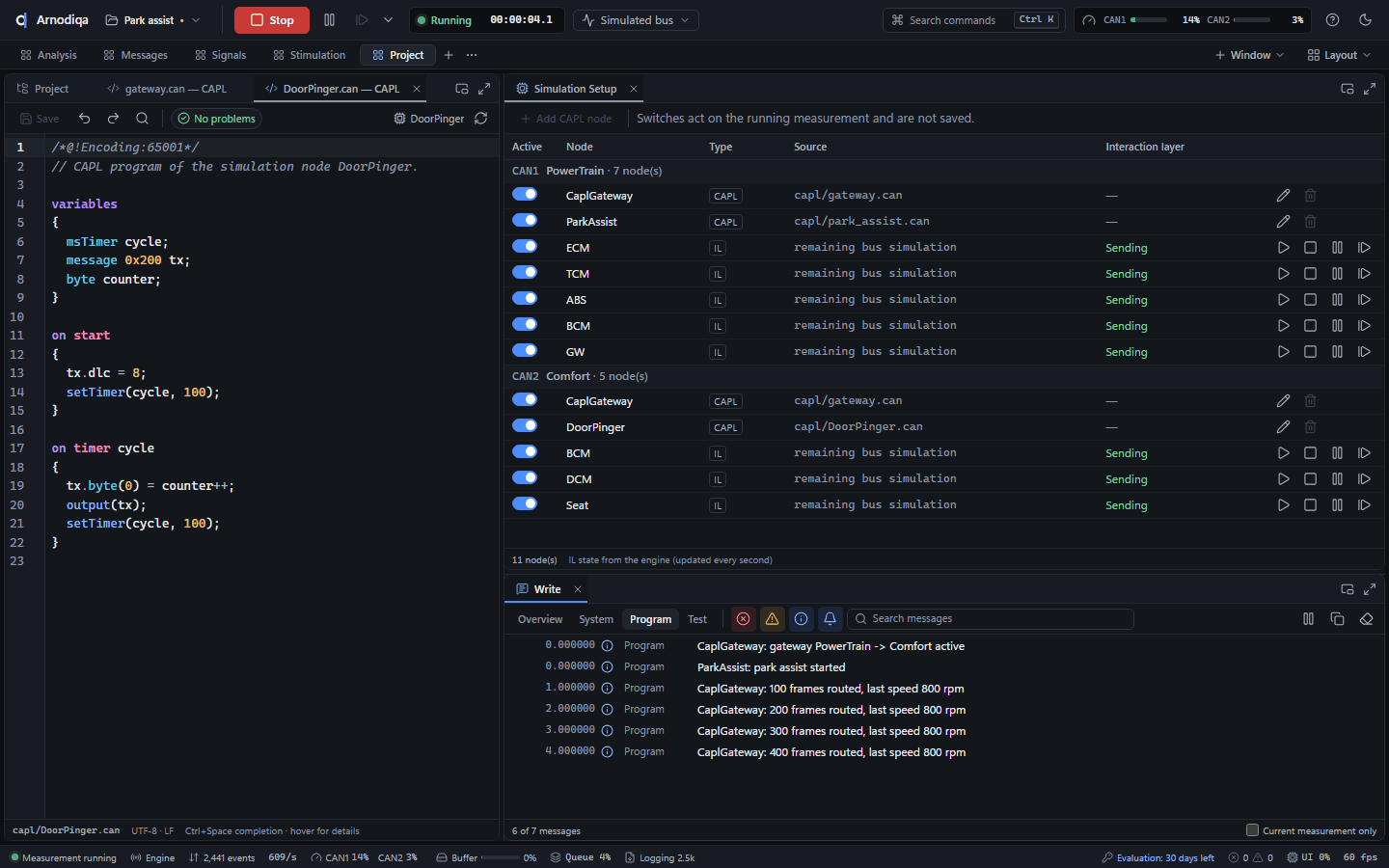
The node appears in the simulation setup and its program opens in the editor. Start the measurement: the CAPL programs run and their write() output appears in the Write window on the Program tab, prefixed with the node name. Save the project to keep the new node.
Run test units in the Test Runner
The Test Runner runs the project's test units on the simulated bus and shows the report in the app. The outcome is the same as with arnodiqa test.
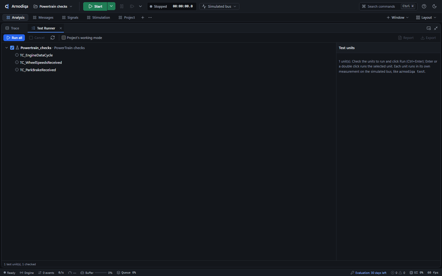
Open the Test Runner with Ctrl+K and New Test Runner window. The left side lists the project's test units (the *.vtestunit.yaml files under tests/) with their test cases; a test tree (*.vtesttree.yaml) appears with its groups. The tick determines which units take part.
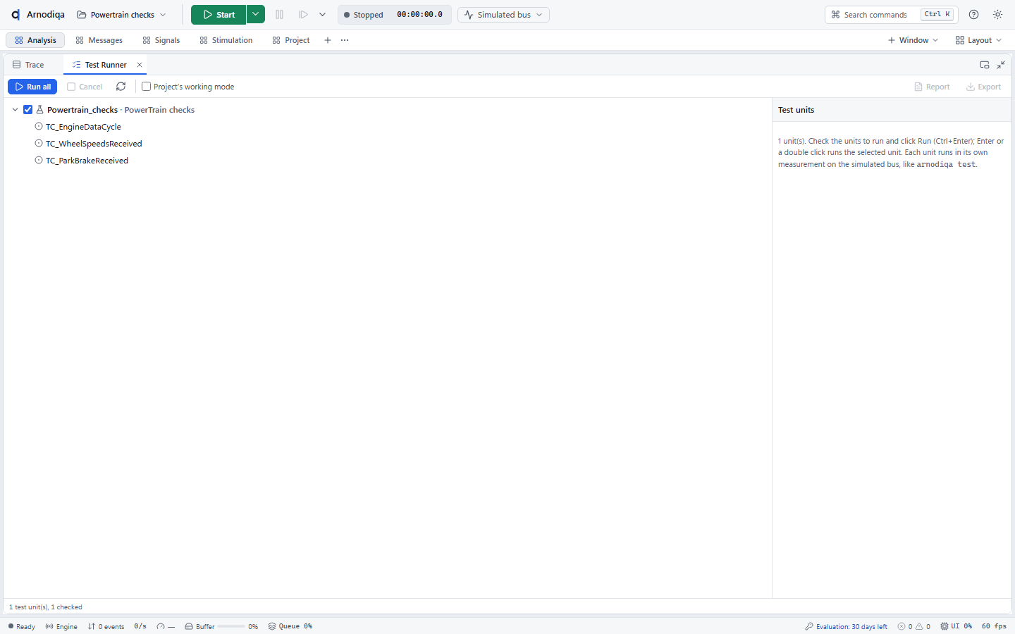
Click a unit for its details: title and description, the file and the CAPL sources (a click opens them in the CAPL Editor). The arrow keys move through the tree, Space toggles the tick and Enter or Run this unit runs the selected unit.
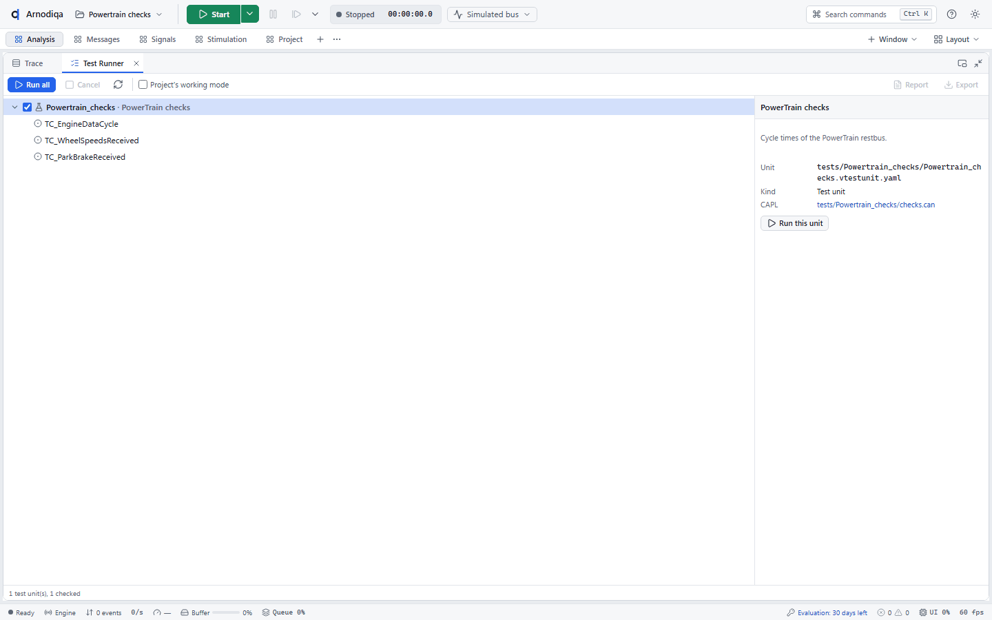
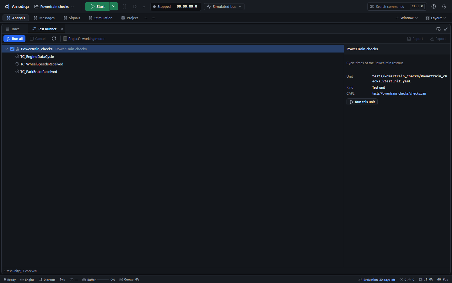
Click Run (Ctrl+Enter). Each unit runs in its own measurement on the simulated bus; the current test case shows Running and the verdicts appear as soon as a test case finishes. Cancel aborts the run: the current unit stops and the rest is skipped.
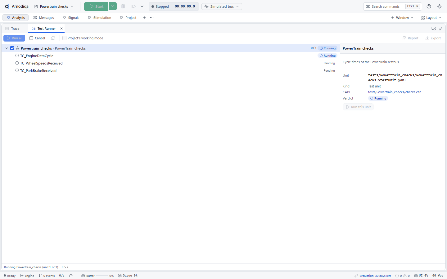
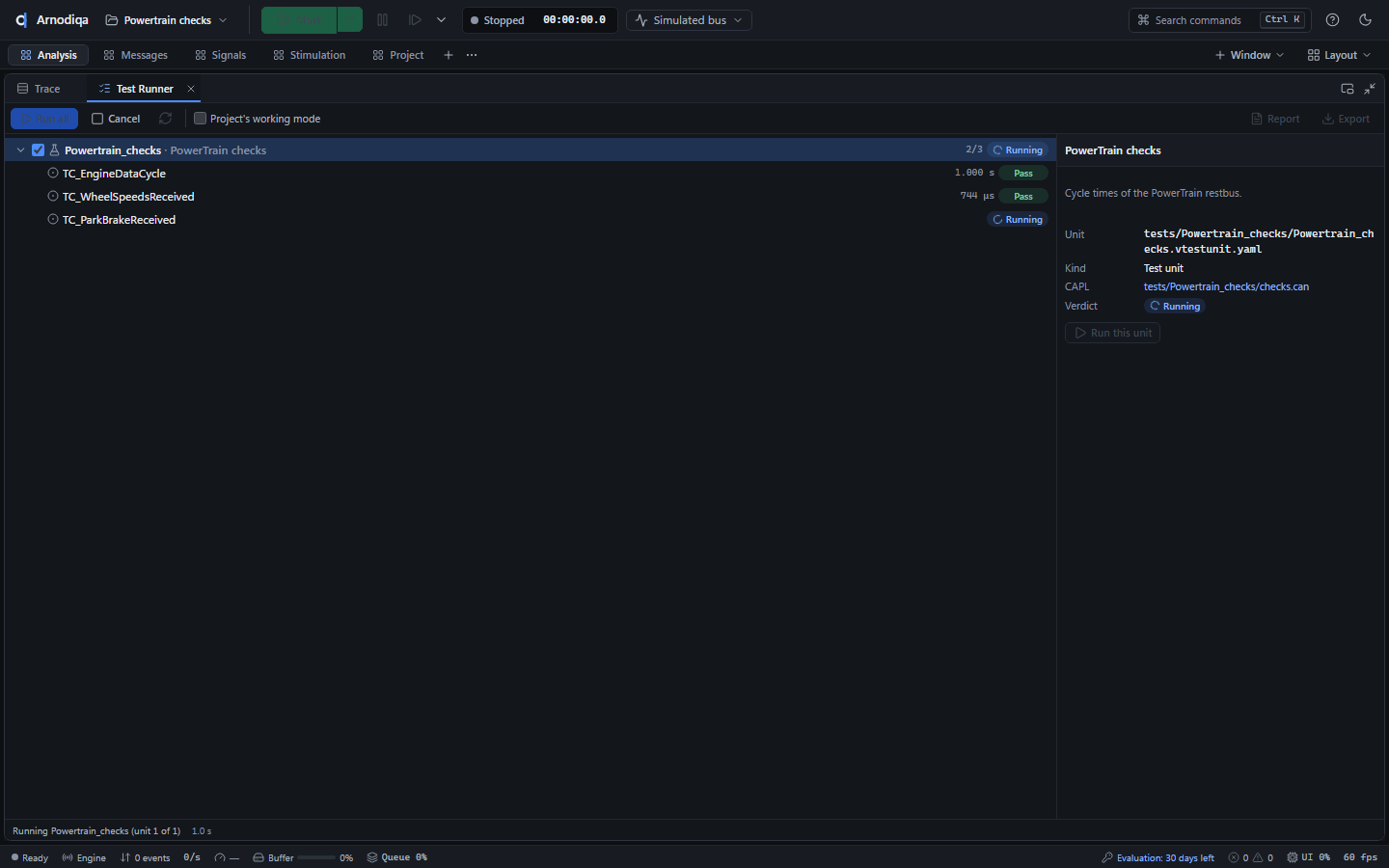
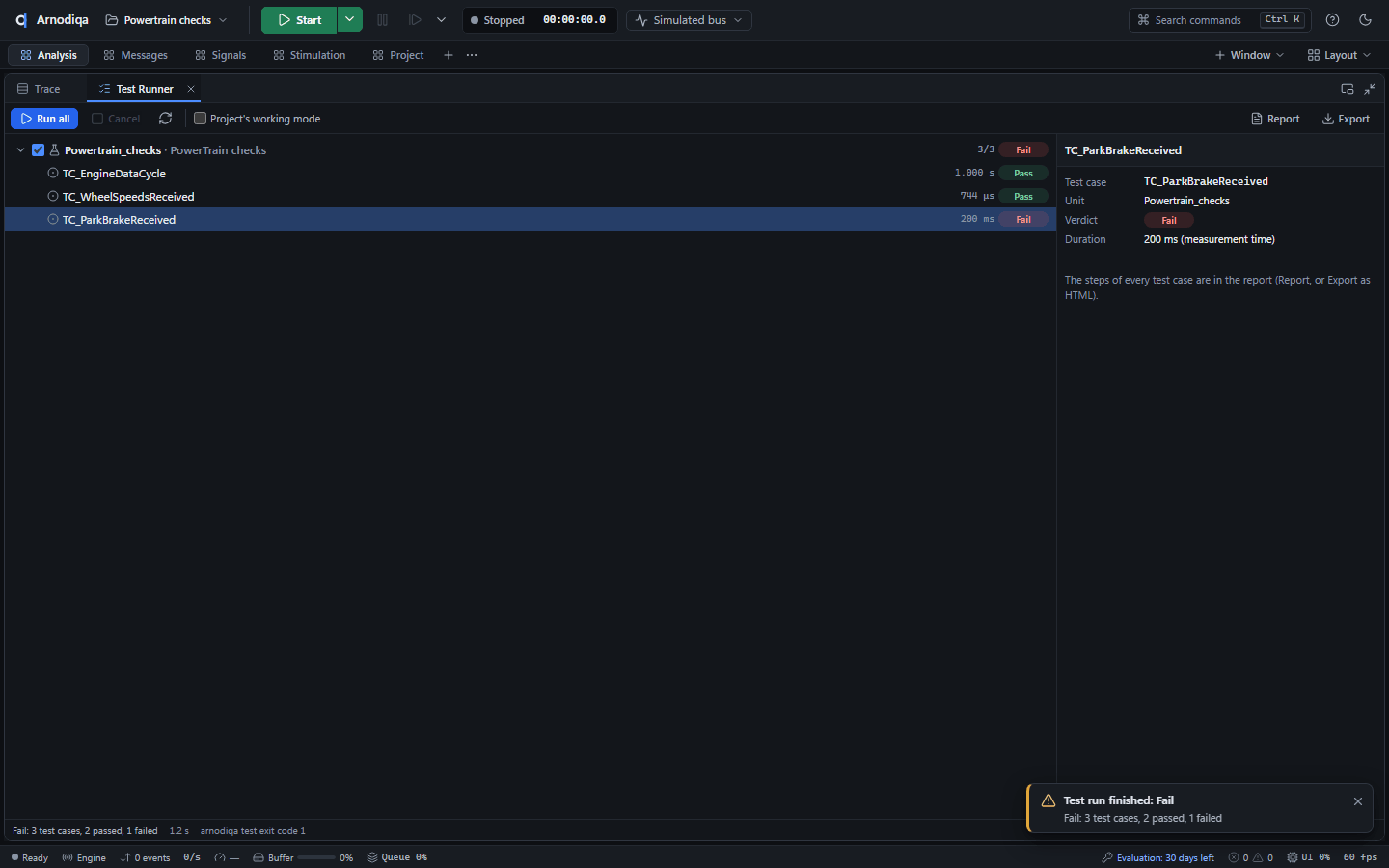
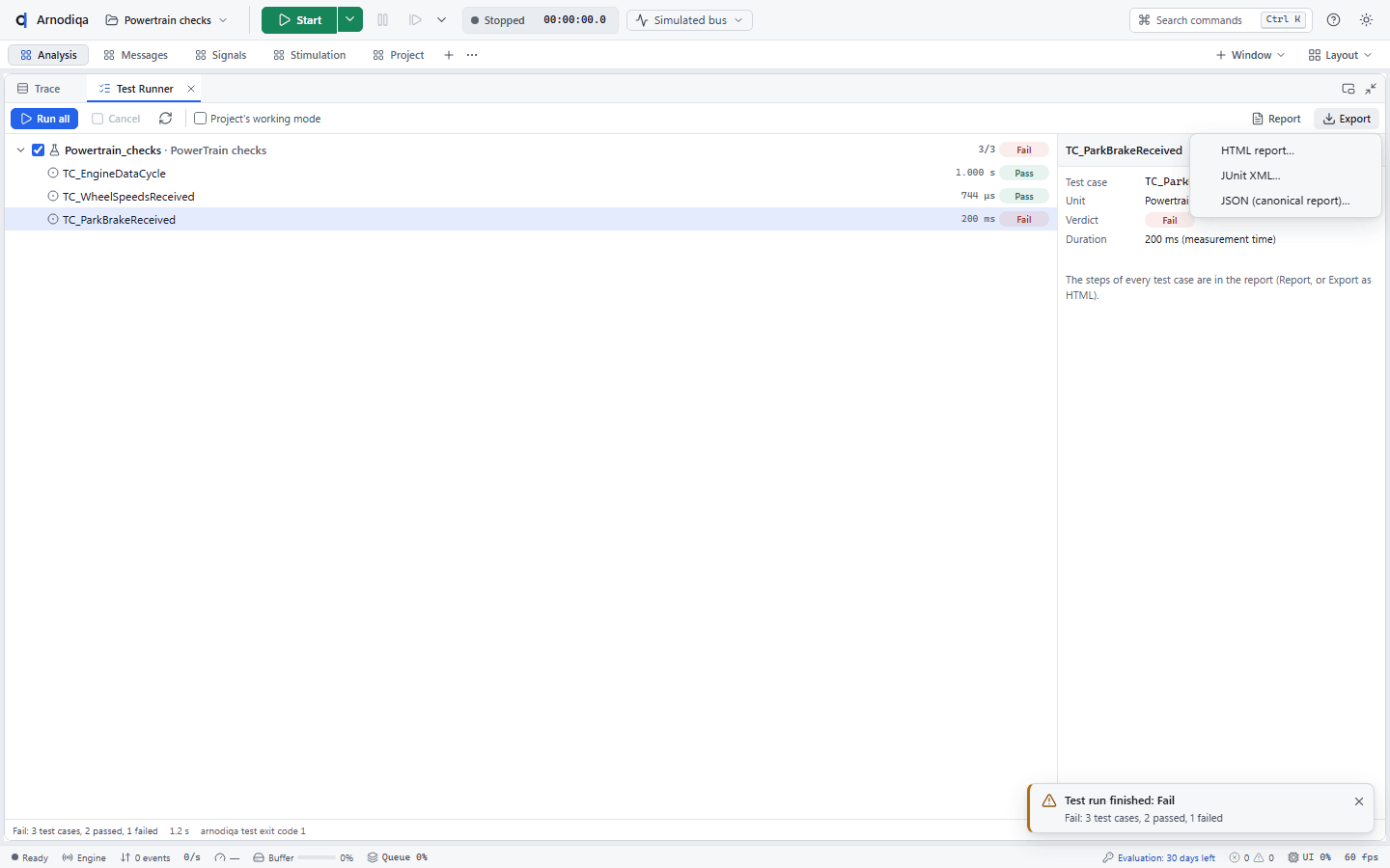
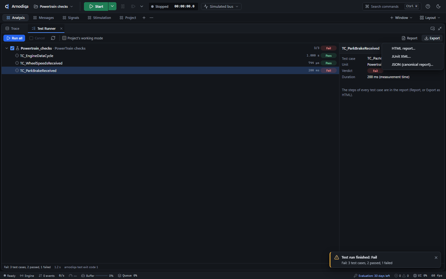
After the run each test case has its verdict (Pass, Fail, Inconclusive, Error) and its duration in measurement time. The bottom shows the summary and the exit code that
arnodiqa testreturns for the same outcome, here 1: at least one test case failed.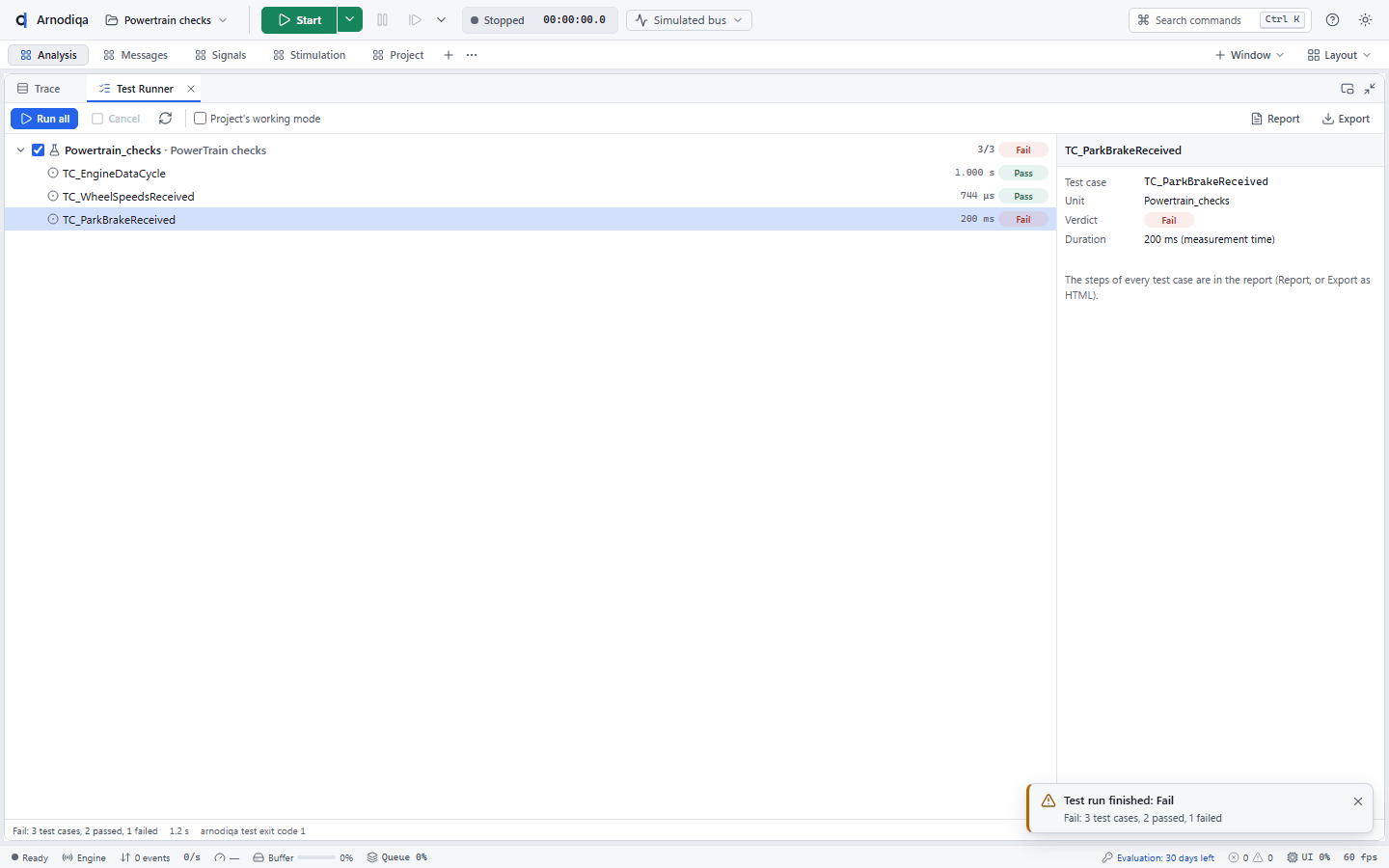
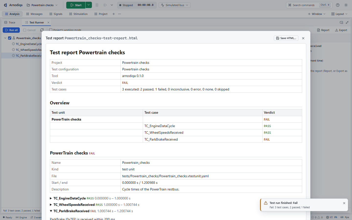
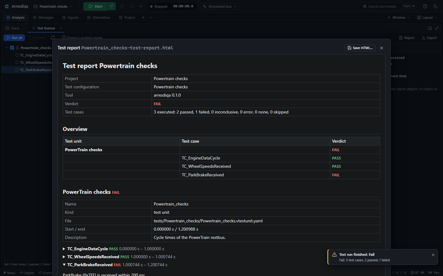
Click Report for the HTML report in the app: information per unit and the steps per test case; failed test cases are expanded. Save HTML… saves the report.
Export saves the report as HTML, as JUnit XML for a CI server or as the canonical JSON report.
LIN: schedule tables, slaves and LIN in the Trace
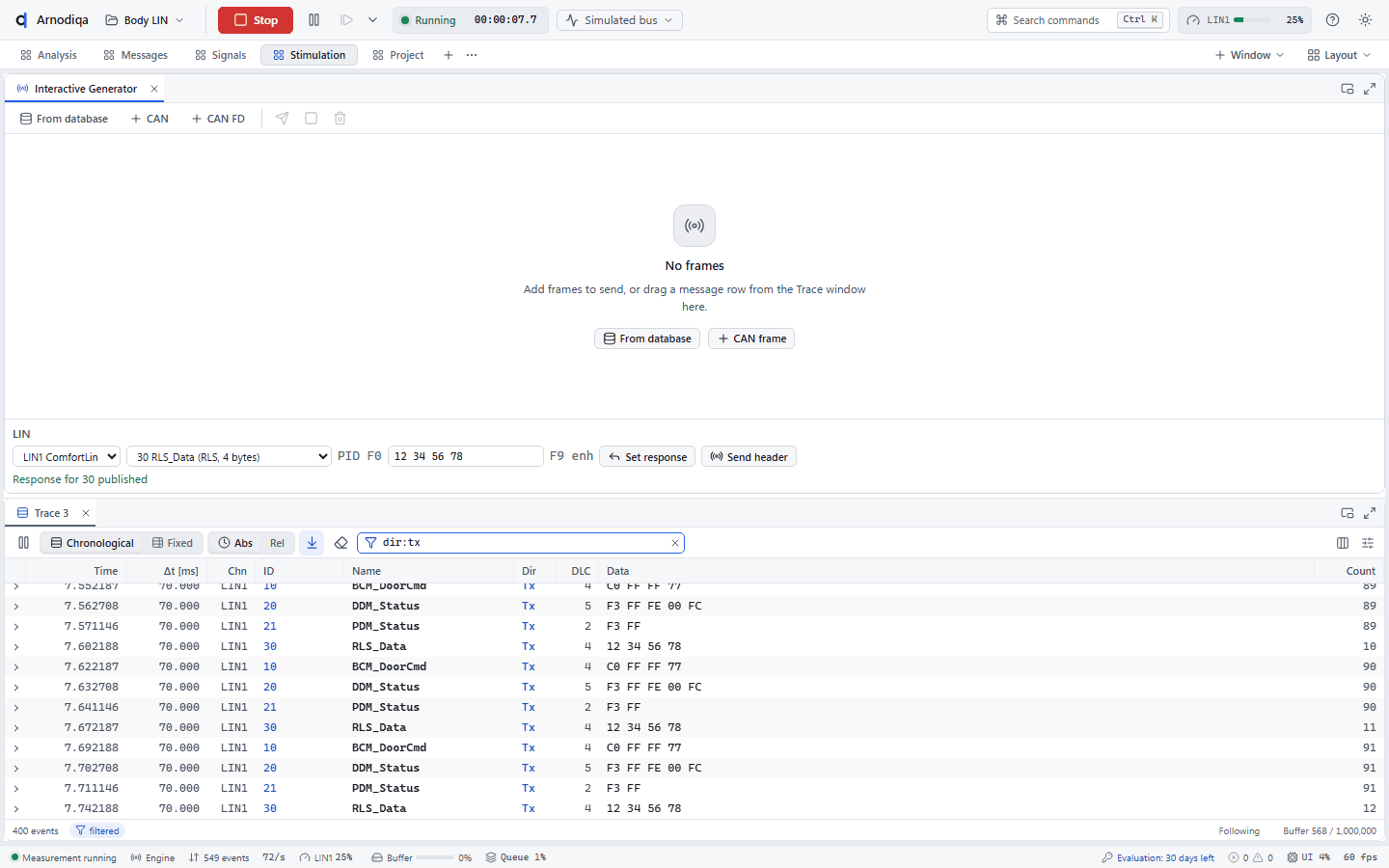
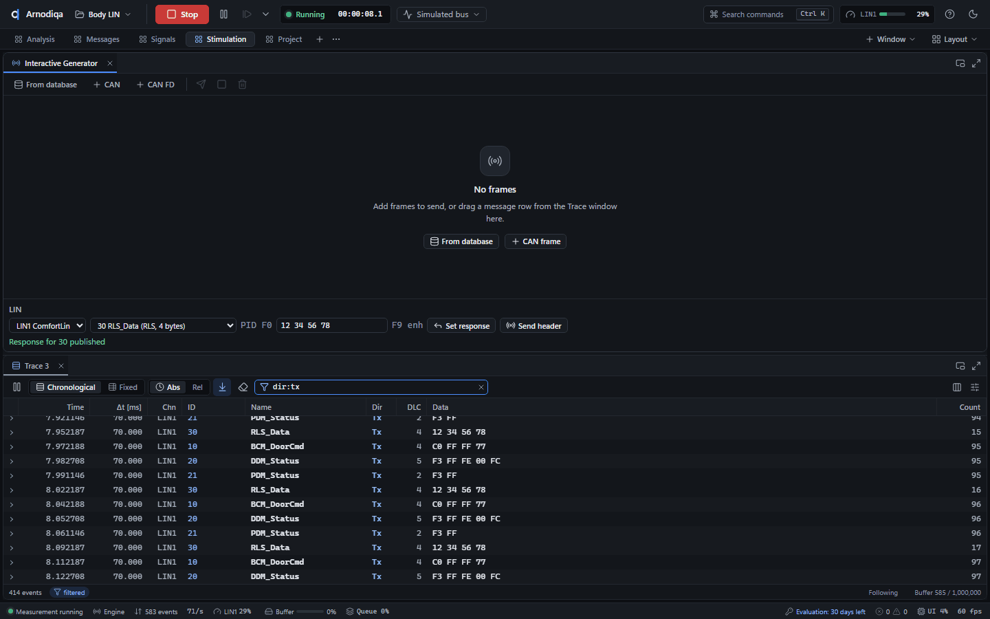
A LIN network comes from an LDF; Arnodiqa simulates master and slaves and shows LIN frames and bus events in the Trace.
Project Body LIN from the LIN cluster template. The project explorer shows the LIN network with baud rate, master, slaves and schedule tables; the simulation setup shows the LIN nodes with their role (master or slave).
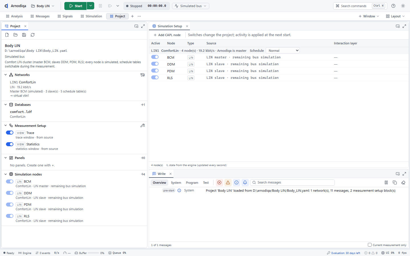
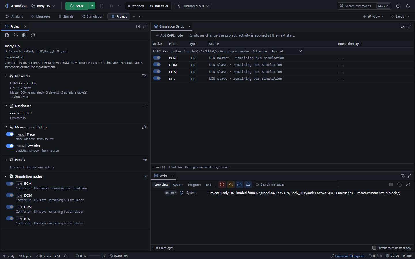
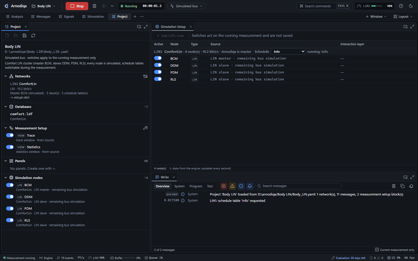
Start the measurement and select another schedule table for the LIN network in the simulation setup. The switch takes place at the end of the running table; the row shows
running: ….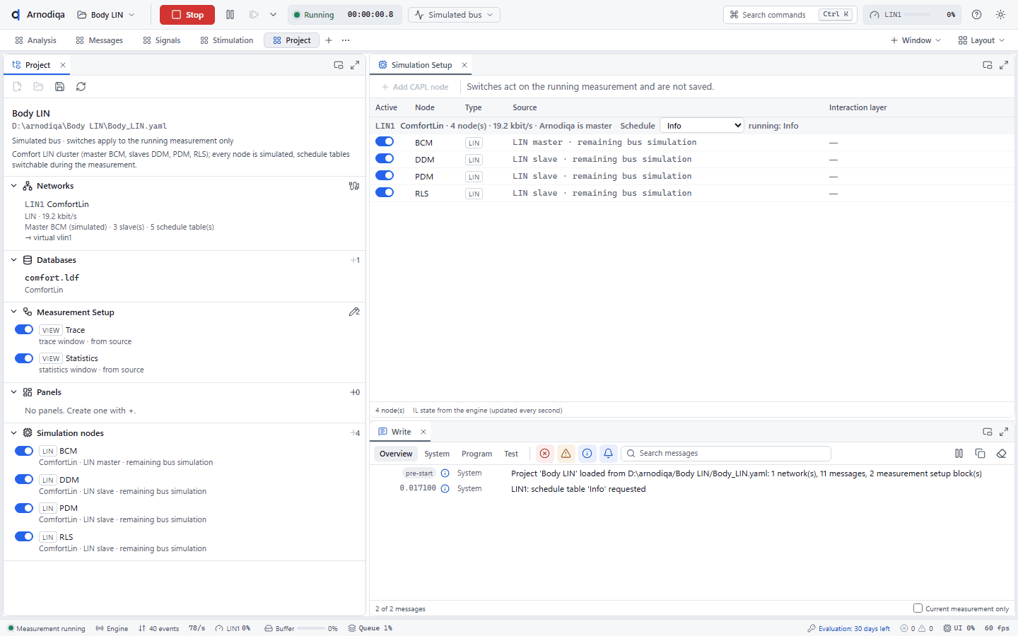
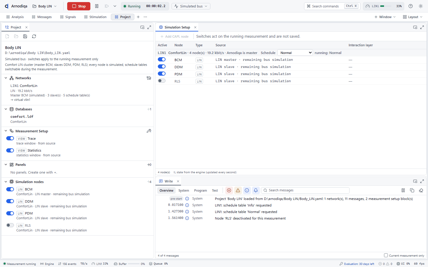
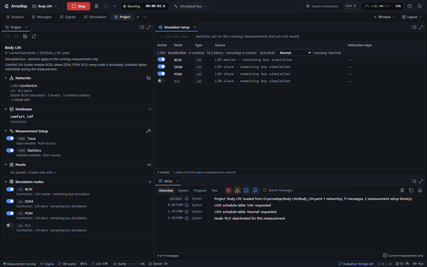
Every slave from the LDF is a simulated node. Turn a slave off with the switch in the Active column (here RLS) to let a real ECU respond in its place. During a measurement this applies to that measurement only; Write then reports Node 'RLS' deactivated for this measurement.
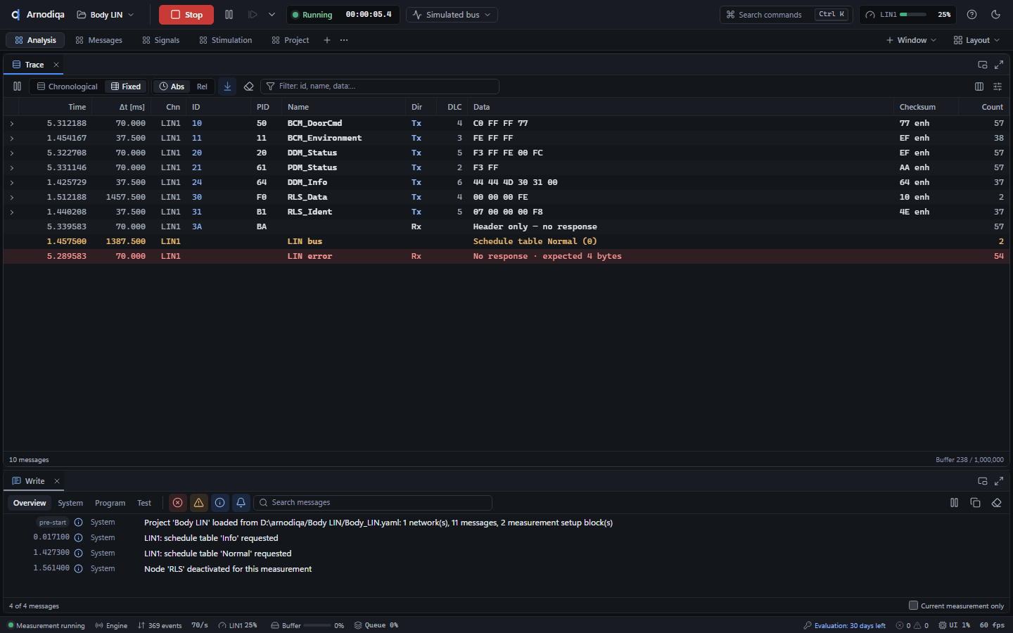
The Trace shows LIN frames on channel LIN1. Use Columns to enable the PID and Checksum columns. Filters:
bus:lin,type:lin,type:linerror(errors) andtype:linbus(wake-up, sleep, schedule change).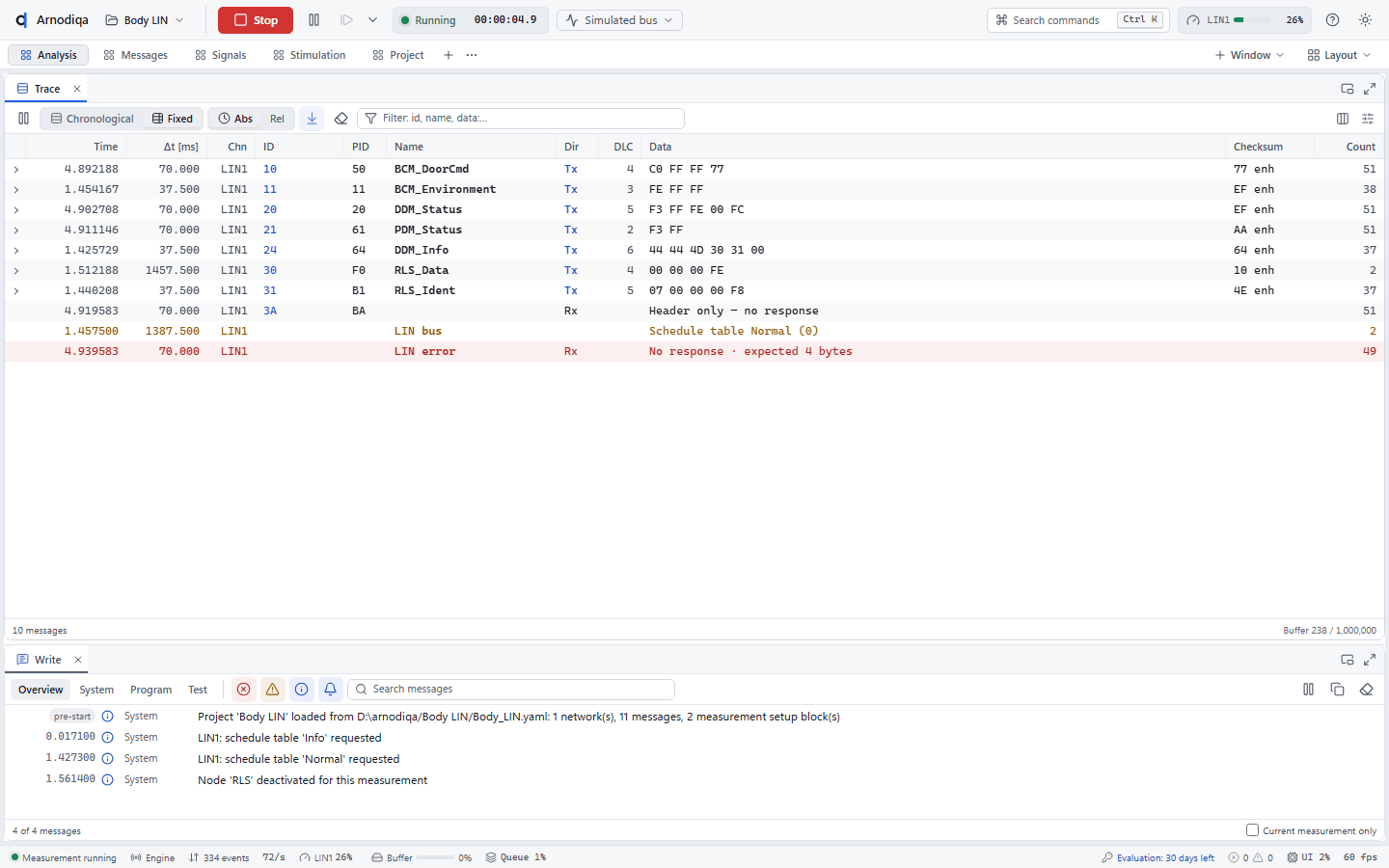
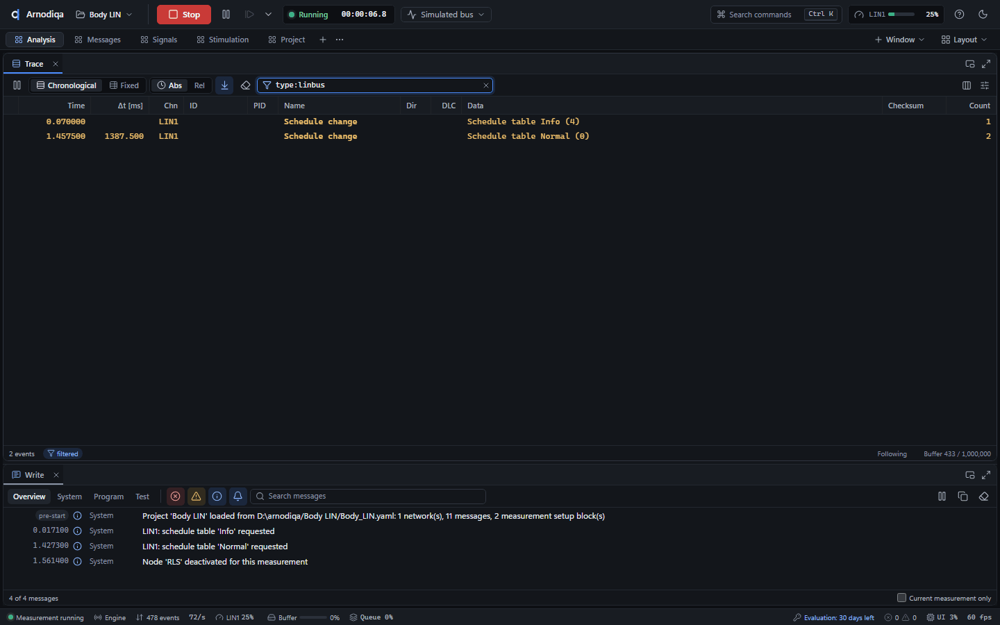
In Chronological mode the filter
type:linbusshows the bus events: here the schedule table changes, and further wake-up and sleep.type:linerrorshows error rows such as No response or Checksum error.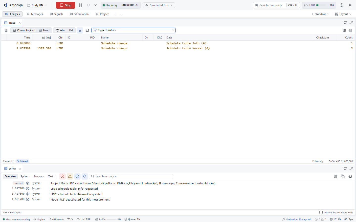
In the Interactive Generator on the Stimulation desktop, select a frame from the LDF in the LIN section. Set response publishes the response as slave, Send header sends the header as master.
J1939 Monitor and DTCs
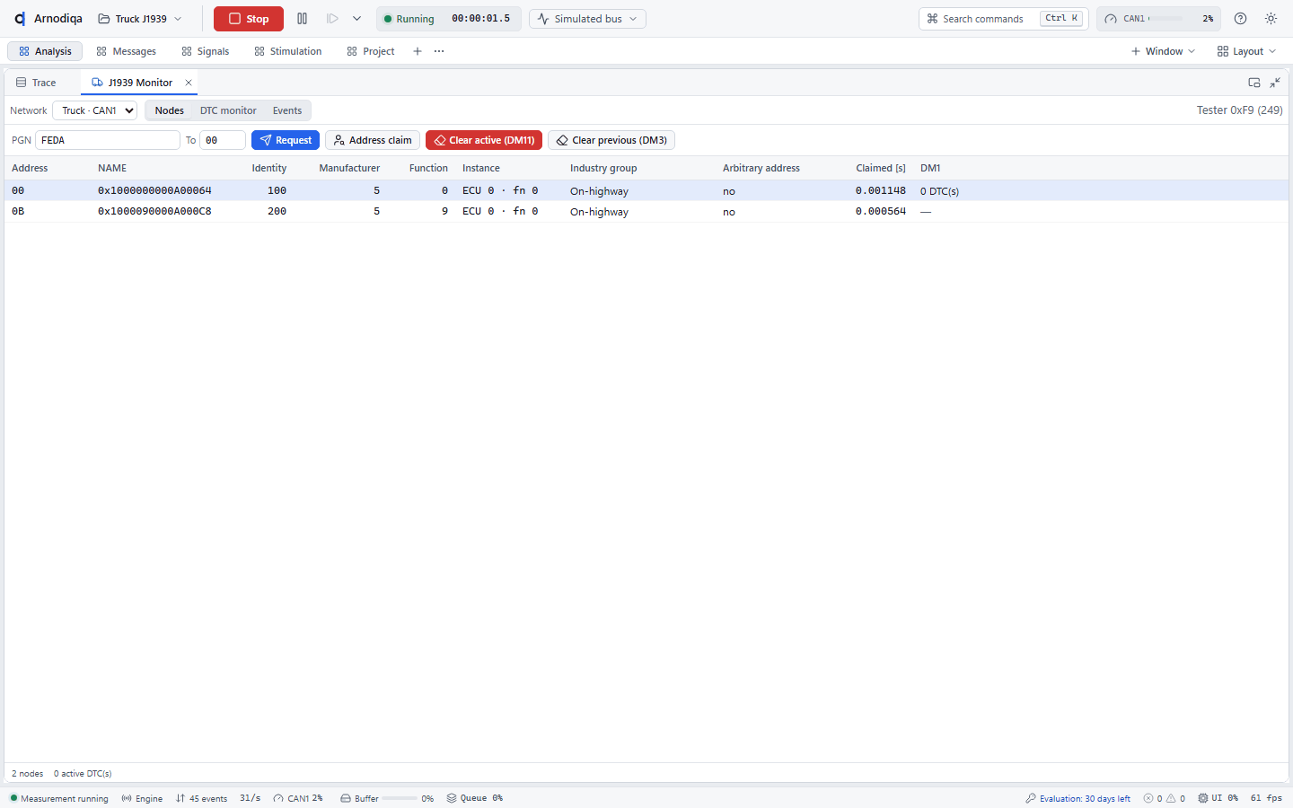
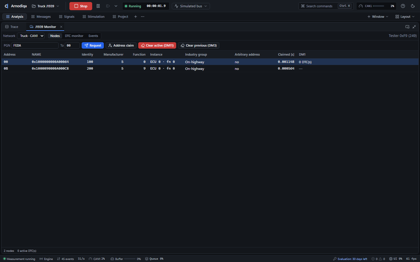
The J1939 Monitor shows the nodes on a J1939 network, their active fault codes and the sequence of claims and transfers.
Open the J1939 Monitor (Ctrl+K, New J1939 Monitor window) and start the measurement. The Nodes tab shows, per address, the NAME with its fields, the time of the address claim and a DM1 summary.
The DTC monitor tab shows the lamps (MIL, RSL, AWL, PL) of each node and the active DTCs from DM1: SPN, FMI with text and the occurrence count.
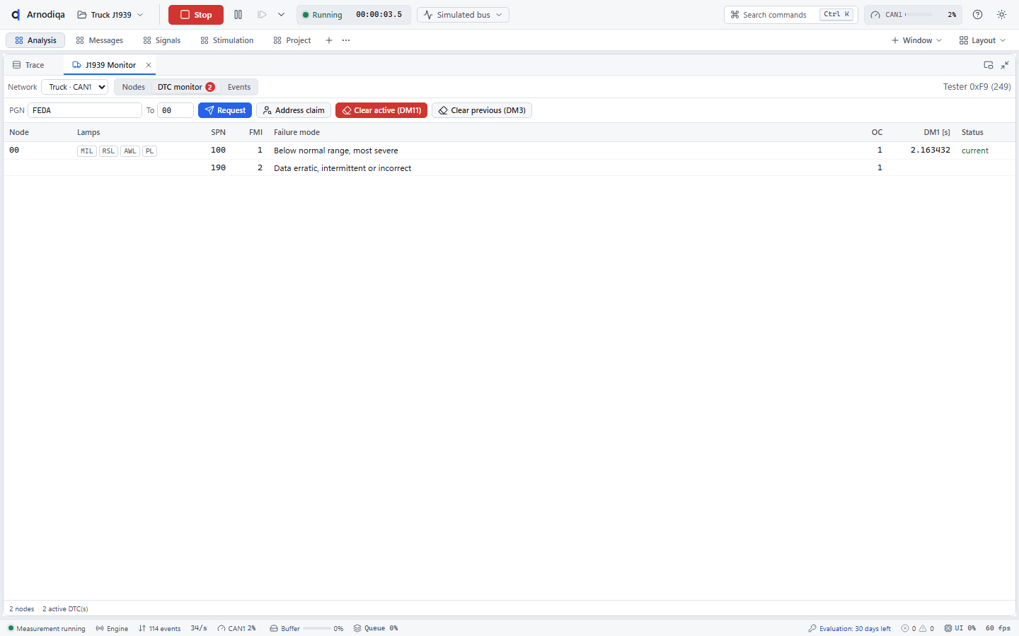
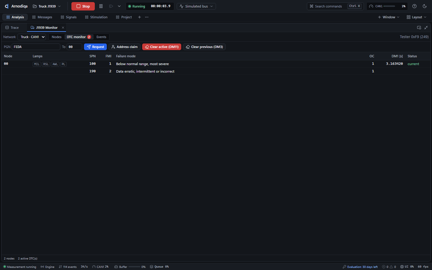
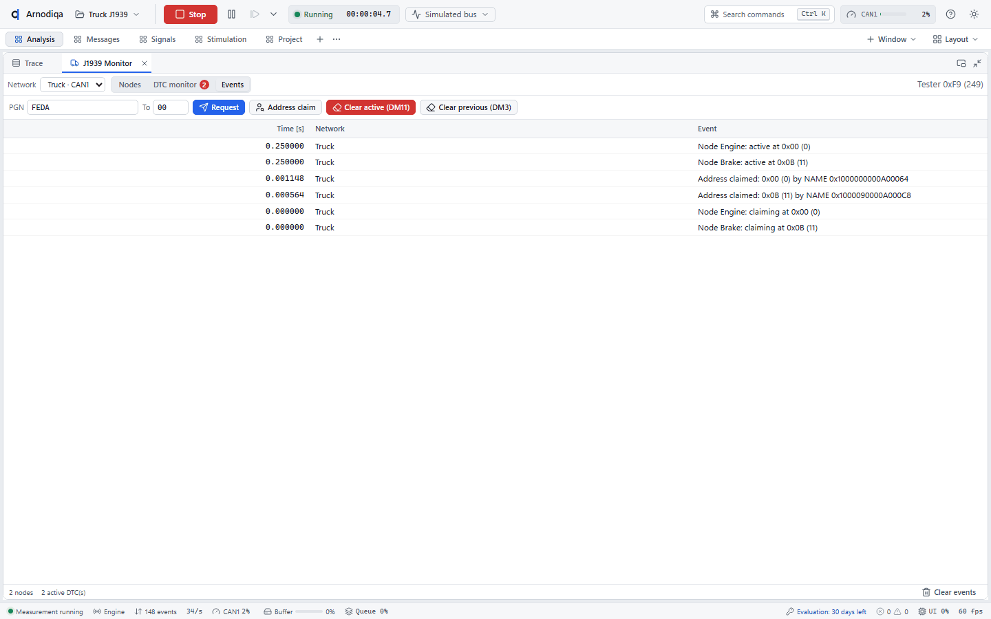
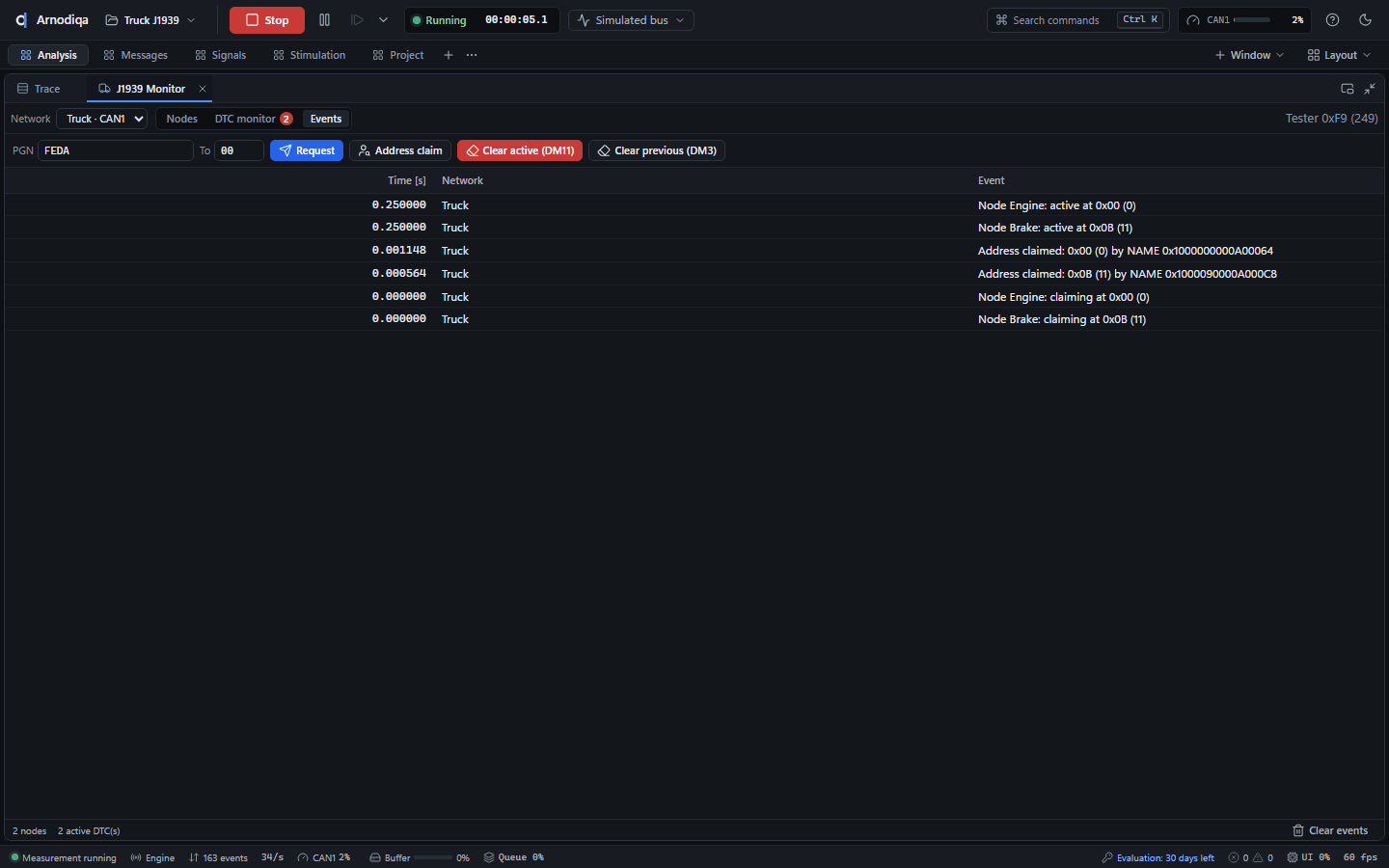
The Events tab shows address claims, requests and responses, ACK/NACK and transport protocol messages. Request requests a PGN from a destination (hex); Clear active (DM11) and Clear previous (DM3) clear DTCs.
Database editor: add a signal
The Database Editor edits the project's DBC and LDF files, with undo/redo and checks while editing.
In the project explorer, click the pencil next to the database (here powertrain.dbc). The Database Editor shows the tree on the left (nodes, messages, signals, value tables), the table in the middle and the properties on the right.
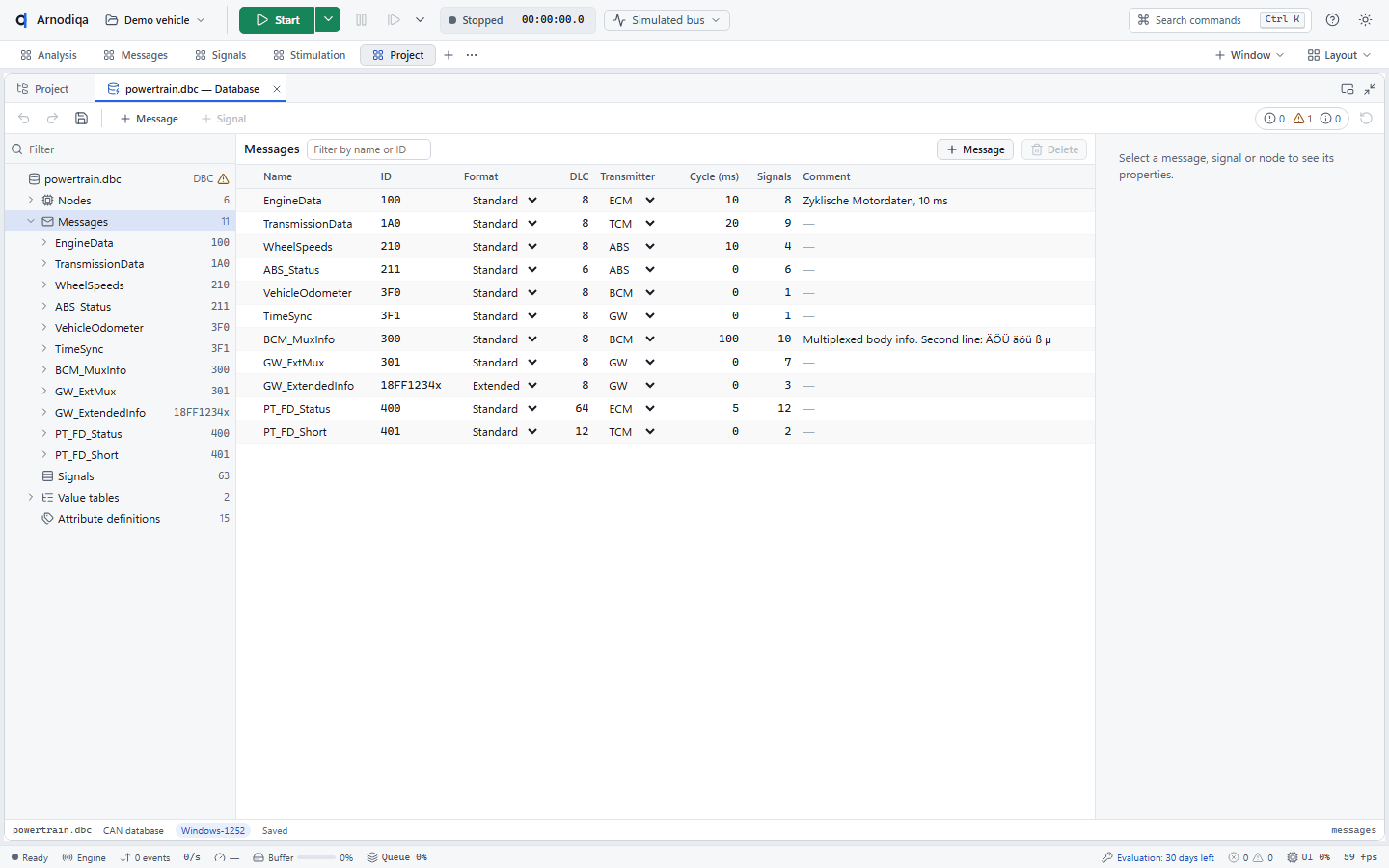
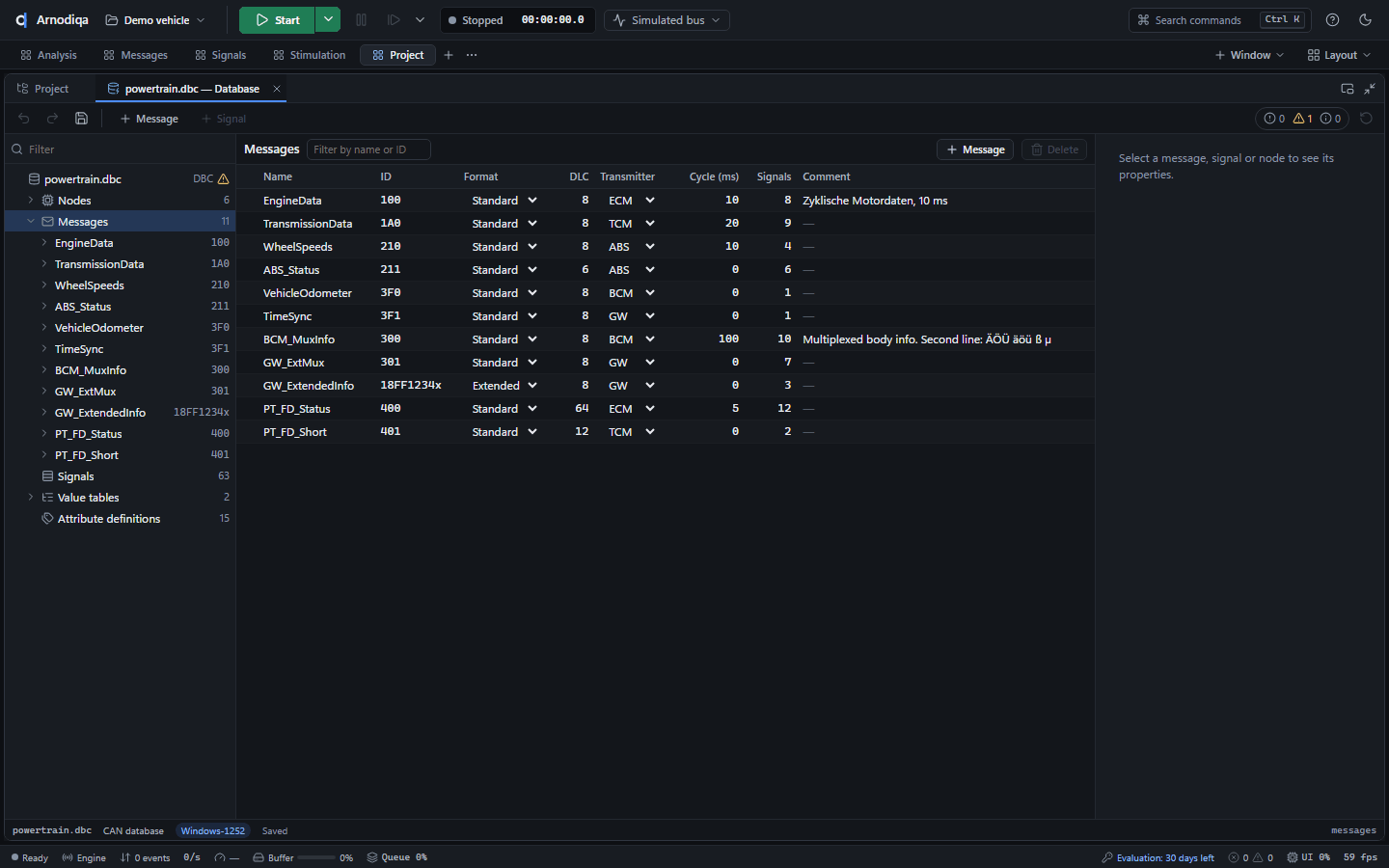
Click a message in the tree (here ABS_Status): the middle shows the bit layout with each signal as a coloured bar, and below it the signals in a table.
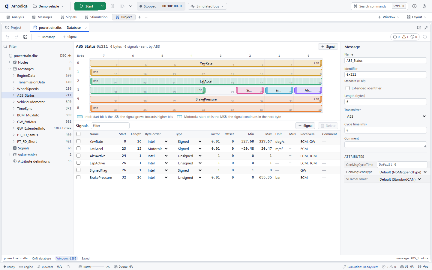
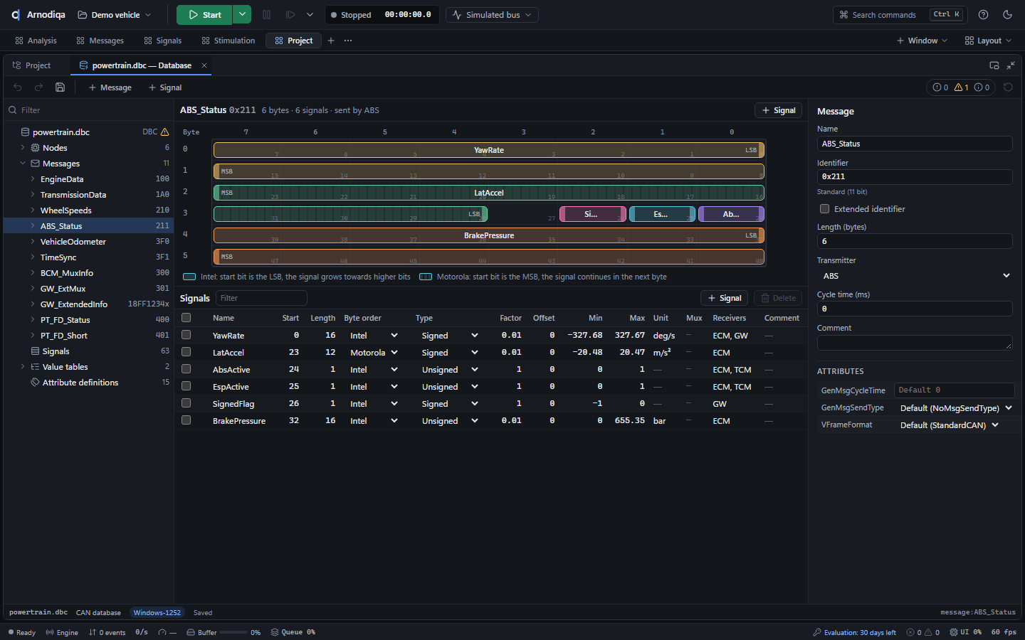
Click + Signal above the bit layout: the new signal (1 bit) is placed at the first free position, here bit 27. Name it on the right under Signal (here BrakeLampOn) and set length, byte order, factor, unit and receivers as needed. Drag the bar to move the signal or an end to change its length; overlaps are marked red.
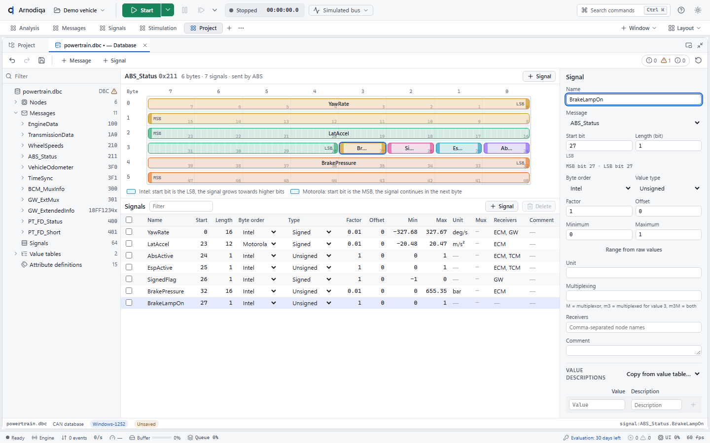
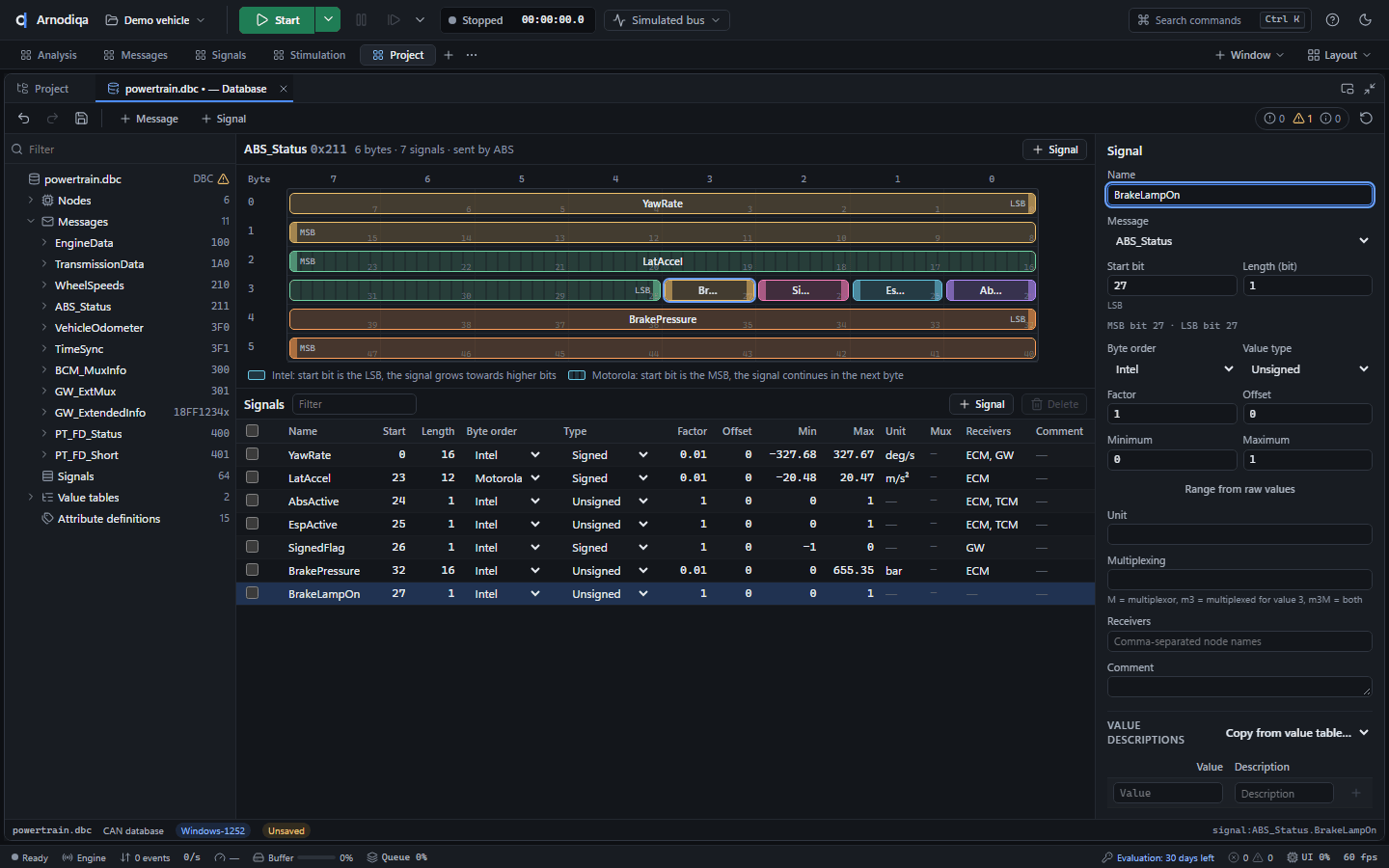
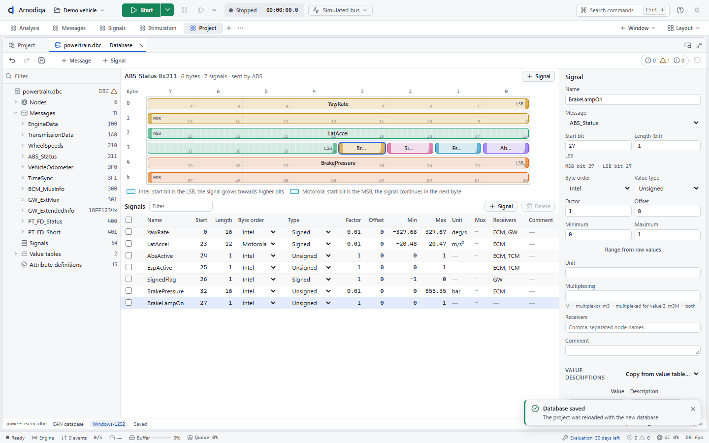
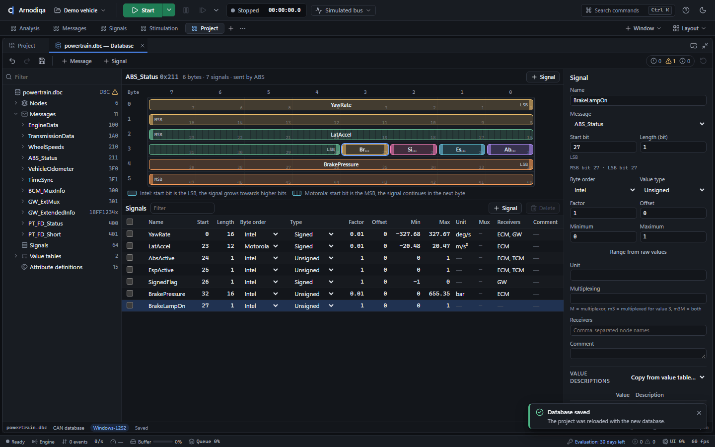
After saving, Arnodiqa reports Database saved and reloads the project with the new database; the Trace decodes the new signal immediately. Ctrl+Z and Ctrl+Y (or the arrows at the top left) undo or redo changes.
Hardware self-test
The self-test checks an interface and its driver with a channel pair or with one channel and internal loopback.
Open the Hardware window (Ctrl+K, New Hardware window or via the project explorer) and click Self-test…. The icon next to a channel starts the test for that channel only.
Choose the setup: Channel pair (two channels connected by a cable) or One channel, channels A and B, the bit rate, CAN FD and the checks. Without hardware, Try on virtual channels runs the test on a virtual bus.
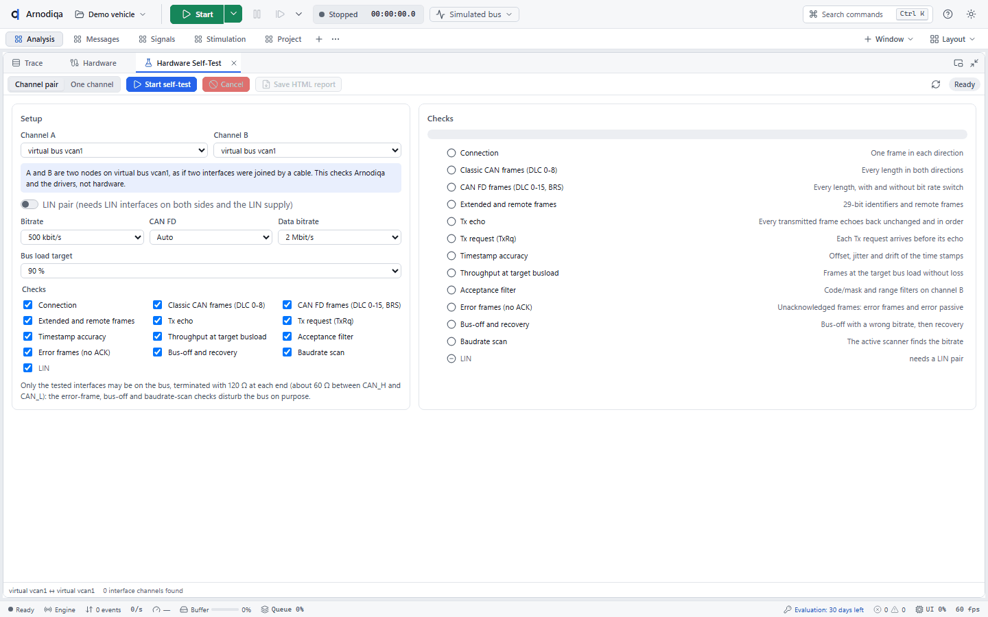
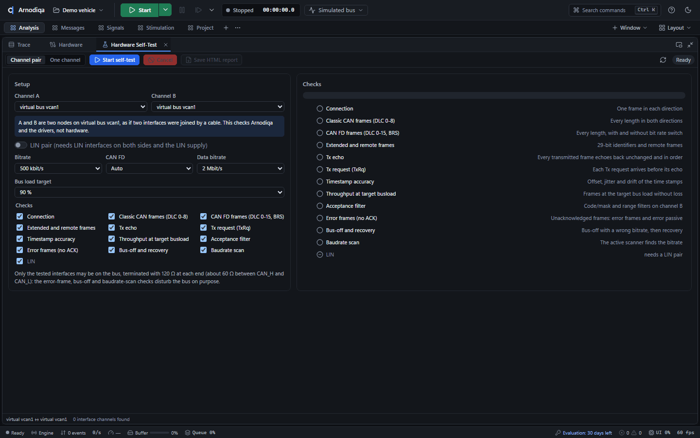
Click Start self-test (Ctrl+Enter). Each check shows its status and duration.
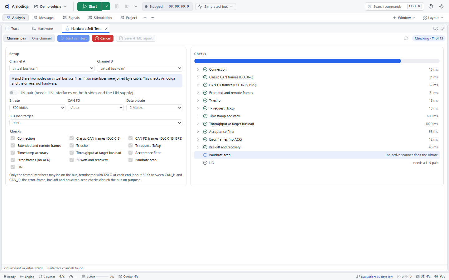
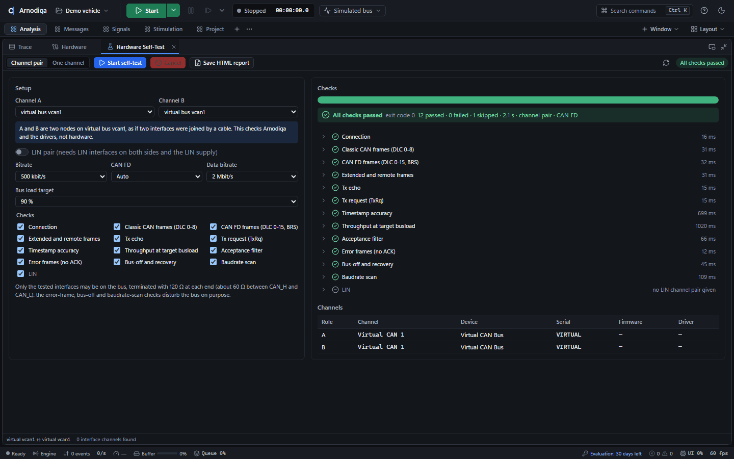
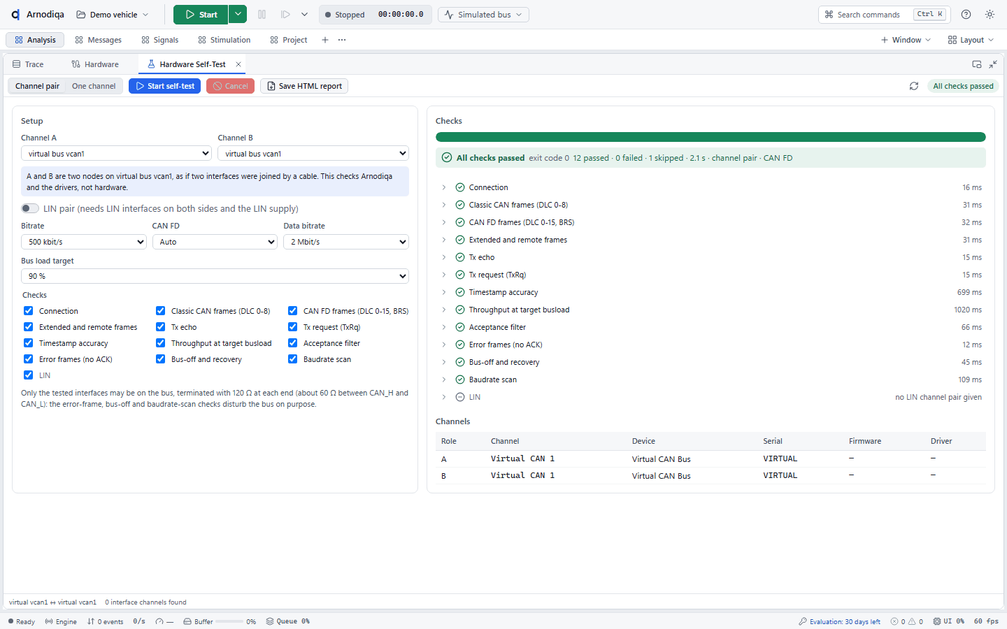
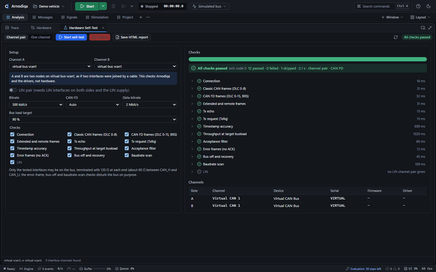
The summary follows, with the channels (device, serial number, firmware, driver). Expand a check for measured values and, on a failure, the likely cause. Save HTML report saves the report.
Support bundle and log folder
Logs and crash reports stay on the computer. You create a support bundle yourself and send it through your own channel to support@arnodiqa.com.
Click the question mark (Help) at the top right. The menu contains Open log folder, Create support bundle…, Debug logging until restart and About Arnodiqa. The same actions are available in Ctrl+K under Help.
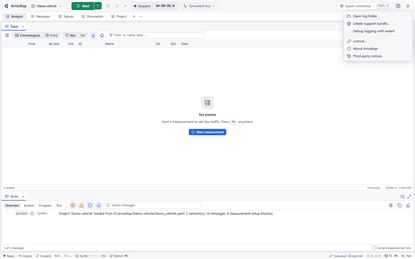
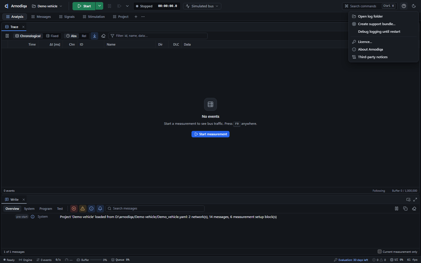
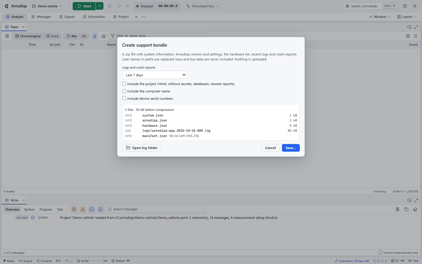
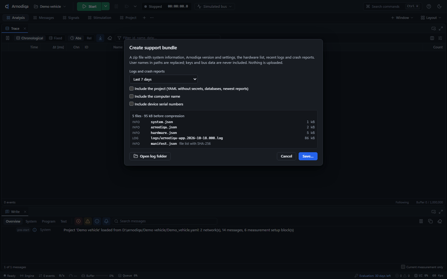
Create support bundle… shows in advance which files go into the zip file and what is deliberately left out. Choose the period of the logs and whether the project, the computer name or serial numbers may be included. Click Save… and choose where the zip file goes; nothing is sent.
Open log folder opens the folder with the Arnodiqa log files in Explorer; a notification shows the path.
FAQ
Can I use it with real hardware?
arnodiqa hw list and the Hardware window show what was found. Arnodiqa uses the manufacturer's official driver; use the Hardware Self-Test to check an interface in your own setup. See hw list.Can I simulate a rest bus?
simulation.restbus every DBC node becomes an interaction layer node with the send types, cycle times, start and inactive values from the database. Exclude the ECU under test with exclude. See Project format.Will my existing CAPL code run?
arnodiqa capl check. The language is implemented from our own specifications.Can I run tests in CI?
arnodiqa test runs the test units of a project on the simulated bus, writes reports as HTML, JSON and JUnit XML and returns an exit code based on the verdict.Are BLF files interchangeable with CANoe/CANalyzer?
Which platforms?
Does it work without internet (air-gapped)?
Do I need a dongle or licence server?
*.arnlic) that Arnodiqa checks locally: no hardware key, no activation, no phone-home. Node-locked, site and volume licences are available. Without a licence Arnodiqa works for 30 days with all features, after which viewing, offline replay, conversion and export remain available. See arnodiqa license and Pricing.